[AM-04-073] Polynomial Functions

Gimond, M. (2025). Polynomial Functions. The Geographic Information Science & Technology Body of Knowledge (2025 Edition), John P. Wilson (ed). DOI: 10.22224/gistbok/2025.1.10

1. Why Fit a Polynomial Function to Spatial Data?
2. What Are Polynomial Functions?
3. Polynomial Functions in One Dimension
4. Transitioning from a One-dimensional to a Two-dimensional Space
5. Evaluating a Model’s Goodness of Fit
6. A Note about Adopting Traditional Statistical Measures of Significance to Spatial Functions

 

1. Why Fit a Polynomial Function to Spatial Data?

Fitting a polynomial model to spatial data may serve different purposes. For example:

• In the interpolation of sampled locations (Unwin, 1981);
• In understanding the relationship between a variable and its location (James et al., 2013)
• In de-trending the data for:
  • Revealing localized patterns in the data masked by dominant trends (Haining, 2004);
  • Satisfying requirements in some analytical procedures that make use of modeled variograms (e.g., Kriging interpolation techniques) (Bailey & Gatrell, 1995).

Fitting a trend to the data only makes sense for spatially continuous fields–an entity that can be measured anywhere within the study extent using ratio or interval scales (O’Sullivan & Unwin, 2010). Examples of spatially continuous data include precipitation, population density, elevation, median county income, etc. It does not make sense to fit a trend to discrete features such as the location of crime events or the distribution of trees.

While the variable of interest needs to be continuous, it can be made available in any different spatial data model such as point, contiguous polygons or raster. For a point data model, the observations are to be treated as sampled observations of the underlying phenomena in which case a polynomial function is used to interpolate the data at unsampled locations. In this topic, polynomial functions will be explored using a raster data model but note that the method for fitting a polynomial function highlighted here is applicable to different data models.

 

2. What Are Polynomial Functions?

Polynomial functions are mathematical models that seek to describe global trends in a dataset using the general form: 

Equation 1 

  

where zi is a scalar of interest (e.g., precipitation, income, elevations, etc.) and si denotes location in one, two or n-dimensional space. The term β is the model coefficient we are seeking. The term ε refers to the residuals, i.e., parts of the observed data not accounted for in the model (sometimes described as the error term in the field of statistics). The subscript i reminds us that the value z and its residual are a function of location i.

Equation 2 

Here, the ellipsis “…” is a placeholder for higher order polynomial values and interactive terms (e.g. ).

Fitting a polynomial function requires two steps: (1) defining the model (in this case the polynomial order)–this can be linear, quadratic, cubic, quartic, quintic, etc., (2) then fitting the model to the data using, for example, ordinary least squares regression methods (Montgomery et al., 2007).

Because the distances in x and y directions are assumed to be in the same dimension and scale (i.e., a unit change in x is equal to a unit change in y), it is best to work off a projected (aka cartesian) coordinate system. Hence, the projected coordinates system should do a decent job in preserving distance within the study extent. This can limit the study extent to relatively small areas of the earth surface.  

 

3. Polynomial Functions in One Dimension

It may be best to first explore a polynomial function in one dimension. In what follows, we will work with the distribution of 2020 total precipitation (in mm) for the state of Kansas (USA). Figure 1 shows a raster representation of the data. But first, we will explore the spatial trend in precipitation along the bottom row of pixels which will provide us with the one-dimensional (east-west) dataset.

 

The left-hand panel of Figure 2 is a scatter plot of the precipitation values along the east-west gradient. Each point represents precipitation values at each pixel location.

 

The simplest model that can be fitted to the data is the mean precipitation value–a constant. It can be visualized as a horizontal line (left panel of Figure 2). This is also known as a 0th order polynomial model where:

Equation 3

Here,  is nothing more than the mean precipitation value (756.8 mm in our working example). Recall that we are only focusing on the east-west precipitation values hence the y coordinate value is ignored in equation (3).

While such a simple model may not prove useful in modeling trends, it serves as a reference for how well other polynomial models perform. Model evaluation will be addressed later in this chapter.

It is clear from the plot that the precipitation is far from constant across the east-west slice of the data. It shows a distinct upward trend that may be better represented using a sloped line. We can modify the above model by augmenting the polynomial order:

Equation 4

While advanced techniques like generalized least squares and shrinkage methods (e.g., lasso and ridge regression) offer potential advantages, their adoption in the field of spatial analysis remains limited. For this reason, we will primarily use the more widely adopted ordinary least squares (OLS) method (Montgomery et al., 2007) in the following examples.

The OLS method seeks to minimize the squared distance between the points and the fitted model when measured parallel to the y-axis in the scatter plot. The left-hand panel of Figure 3 shows those distances using red colored line segments.

 

The distance between the modeled line and each precipitation value is the residual (εi). This is part of the data not accounted for in the model.

Fitting the first order polynomial to the data gives us the coefficients of 305.8 and 1.6 for β0 and β1 respectively.

The  coefficient tells us that for every km increase in the (positive) x direction, precipitation increases by 1.6 mm. Note that the interpretation of the coefficient is dependent on the mapping units used. Typically, projection units are in meters or feet. But, when working at a scale like the State of Kansas, it is best to report changes in value as a function of larger mapping units such kilometers or miles.

Statisticians will seldom stop here when fitting a model to the data. It is good practice to plot the residuals against the x value. This diagnostic plot is useful in assessing if the overall trend in the data was properly characterized by the polynomial model. To help guide our eyes, we add a non-parametric curve to the data which does not make any assumptions about the pattern in the data. Here, we make use of a loess fit, but note that many other non-parametric models can be used for this purpose (Right-hand panel of Figure 3).

The diagnostic plot suggests that the first order polynomial model we adopted does not fully capture the overall trend in the data. There appears to be some curvature in the residuals. This may suggest that we increase the polynomial order by an extra degree.

A second order polynomial model in a one-dimensional space takes the form:

Equation 5

This model generates a curved fit often called a quadratic model (Left-hand panel of Figure 4).

 

The residual diagnostic plot for this model shows a significant improvement in that the non-parametric fit (dashed blue line) does not show an overall trend in the data suggesting that a second order polynomial model is a good fit for our data (Right-hand panel of Figure 4).

A unique characteristic of spatial data is the presence of autocorrelation which is very much apparent in both the original scatter plot and the diagnostic plot. One might be tempted to try and capture this non-random pattern in a polynomial model. For example, fitting a 20th order polynomial model would do a decent job in capturing both the overall trend and localized variation as shown in Figure 5.

 

But, doing so is ill advised–the model has 20 coefficients! Polynomial models are intended to capture general trends in the data. There are more sophisticated and specialized statistical methods used to capture localized spatial autocorrelation. A general rule of thumb is to avoid going above a 3rd order polynomial model unless there is compelling evidence to do so. Any higher order model is likely to capture some aspects of spatial autocorrelation.

 

3. Transitioning from a One-dimensional to a Two-dimensional Space

The polynomial functions described in the earlier section can easily be extended to a two-dimensional space. Next, we fit polynomial functions to the full precipitation extent for the state of Kansas. This adds the y-coordinate variable to the model.

We learned that the 0th order polynomial is a horizontal line in one dimensional space. For a two-dimensional space, this is a horizontal plane that can be defined as:

Equation 6

where  is the mean precipitation for the entire study extent–660 mm in our working example. Figure 6 shows this plane in a three-dimensional space.

 

An east west trend is apparent in the three-dimensional scatter plot suggesting that we should seek a first order polynomial, at the very least. The model takes on the form:

Equation 7

The model defines a plane that can be tilted in any direction. As was the case with the one-dimensional dataset, we can leverage the least squares method to fit the model to the data. This results in the following coefficients:

Equation 8

The coefficients tell us by how much the precipitation changes along the x and y coordinate directions. In our working example, precipitation increases by 1.15 mm in the x direction (west to east) and decreases by 0.45 mm in the y direction (south to north). The precipitation gradient is greater in the x-direction than in the y direction. Figure 7 shows a three-dimensional rendering of the plane.

 

The same model can be viewed as a two-dimensional raster where each pixel represents the modeled precipitation (Top panel of Figure 8).

 

How well does the first order polynomial fit our data? We may first want to look at the residuals (Bottom panel of Figure 8). The overall trend observed in the original raster is no longer obvious. However, subtle trends are more difficult to make out when viewing a two-dimensional dataset than a one-dimensional dataset. A more effective way to assess model fit in two-dimensional space is to split the residuals into their x and y coordinate components by plotting the residuals as a function of x and y respectively (Figure 9).

 

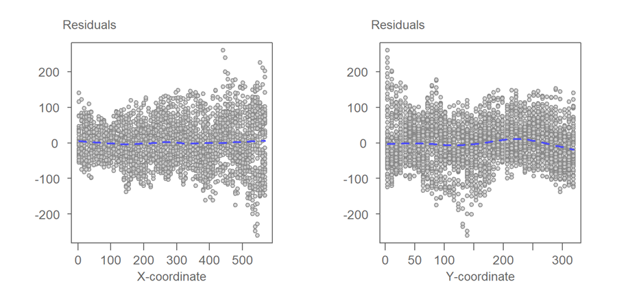
The plots suggest a very mild curvature in the residuals along the x coordinate. A similar, but more complex curvature can be observed along the y-coordinate. It may be worthwhile to augment the function by another polynomial order giving us a second order polynomial function to see if it removes some of these trends. Such a function is also called a quadratic polynomial function. It takes on the form:

Equation 9

Note that in addition to adding the squared coordinate values, the function also adds the interactive terms xy. The interaction term captures situations where the coefficients for x or y are no longer a constant. For example, if the effect of the x coordinate value on precipitation changes as a function of changing y coordinate values, then x’s coefficient can no longer be deemed a constant (James et al., 2013).

The least squares method can be used to fit the function to the data. In our example, this gives us:

Equation 10

The top panel of Figure 10 is a raster view of the modeled quadratic surface. The resulting residuals are shown in the bottom panel (a three-dimensional view of the quadratic surface is omitted as the slight curvature would be difficult to discern in a static figure).

The resulting residuals do not look a whole lot different from those of the 1st order polynomial fit. This is, in part, because the residual rasters highlight the localized variability not captured in both models. This point is emphasized in Figure 11 which shows the difference between the 2dn order polynomial residuals and the 1st order polynomial residuals.

 

The difference in residuals covers a range of about 60 mm, that’s about 5% of the total range of precipitation values suggesting a small improvement in predicting precitpiation values. Despite this small improvement, it is worthwhile to assess the goodness of fit by plotting the residuals against the x and y coordinate values (Figure 12).

 

The second order polynomial offers a detectable improvement over the first order polynomial along the x-coordinate axis where the slight curvature observed in the first order polynomial model’s residuals is no longer apparent. Note that the range of residual values are also slightly less for the 2nd order model versus the first order model suggesting that the quadratic model can explain a greater proportion of the variability in precipitation values.

Mathematically, there is no limit to the polynomial order you choose. For example, you could explore a third order polynomial function (a cubic polynomial) or even a fourth order polynomial function (a quartic polynomial). But, doing so increases the chance of overfitting the data. Recall that the purpose of modeling the trend is to capture the data’s overall pattern. Polynomial functions are not well suited to capturing local variability in the data.

One option thatmay help eliminate the need for higher polynomial orders is to transform (aka re-express) the variable zi (Montgomery et al). Transforming the data can render a curvilinear function straight (or flat in a two-dimensional space). Transforming the variable may also be scientifically justifiable. There are many datasets that benefit from a non-linear scale. For example, earthquake magnitudes are measured on a log scale and some count datasets can benefit from a square root transformation.

 

4. Evaluatiing a Model's Goodness of Fit

The diagnostic plots have, so far, been visual. We can adopt a more rigorous and systematic approach to evaluating how well the functions fit the data. A popular statistical measure of “fit” is the coefficient of determination, . It is computed by subtracting from one the ratio of the sum of residuals squared in the fitted model to the sum of residuals squared one would get if we had fitted the mean value (Unwin, 1981).

Equation 11

If the residuals from the model are smaller than those obtained if we adopted the simpler mean model,  ends up being large.  ranges from 0 (no improvement whatsoever over the mean) to 1 (a perfect fit where the residuals from the fitted model are zero). In our working example, the first order polynomial model resulted in an  of 0.87. The second order polynomial resulted in an  of 0.90–a slight improvement over the first order polynomial. Note that the  value is sometimes reported as a percentage as opposed to a fraction.

If a polynomial model is fitted to sampled data (for use in interpolation techniques, for example), an adjustment to the R-squared may be warranted if a higher order polynomial model is chosen, especially if the number of observations is small. The adjusted R-square can be computed from R-square as follows:

Equation 12

5. A Note about Adopting Traditional Statistical Measures of Significance to Spatial Functions

Because underlying residuals are likely to exhibit spatial autocorrelation, traditional methods used to assess “statistical significance” of a model and its coefficient should be avoided. For example, the cluster of low residual values in the eastern part of Kansas is a good indication that spatial autocorrelation is present in our data. If statistical inferences are to be gleaned from surface models fitted to data exhibiting spatial autocorrelation, then geostatistical approaches, such as kriging, should be used to model the residuals (Wilke et al., 2019).

References

- Bailey, T. C. and Gatrell, A. C. (1995) Interactive Spatial Data Analysis. Vol. 413, Longman Scientific & Technical, Essex.
- Haining, R. (2003). Spatial Data Analysis: Theory and Practice. Cambridge University Press.
- James, G., Witten, D., Hastie, T., & Tibshirani, R. (2013). An Introduction to Statistical Learning. Springer Nature Link.
- Montgomery, D. C., Peck, E. A., and Vining, G. G. (2007). Introduction to Linear Regression Analysis, Solutions Manual (Wiley Series in Probability and Statistics). Wiley-Interscience, USA.
- O'Sullivan, D. and Unwin, D. (2010) Geographic Information Analysis, 2nd Edition. John Wiley & Sons, Inc.
- Unwin, D. (1981). Introductory Spatial Analysis, 1st Edition. London, UK: Routledge Publishers.
- Wikle, C.K., Zammit-Mangion, A., and Cressie, N. (2019). Spatio-Temporal Statistics with R. Chapman & Hall/CRC.
Learning outcomes
-
1807 - Define a polynomial function.
Define a polynomial function.
1808 - Summarize how, when, and why to use of polynomial functions for modeling overall spatial trends in the data.
Summarize how, when, and why to use of polynomial functions for modeling overall spatial trends in the data.