[FC-05-016] Areal Operations
Areal operations are core techniques in GIS that enable the measurement, representation, and analysis of area-based features. This entry discusses key aspects of areal operations in geographic analysis, including types of geographic areas, representations, measurements, and operations. Geographic areas can be categorized into four primary region types: administrative, thematic, functional, and cognitive, each reflecting a distinct conceptual framework for organizing, interpreting, and analyzing geographic information. While areal operations most often rely on polygon representations, other forms such as points, lines, rasters, and fuzzy representations may be used or combined, depending on the context and analytical objectives. Measuring geometric properties of areas such as area, perimeter, and shape is foundational to quantifying spatial patterns and processes. Areal operations, including overlay, aggregation, proximity, generalization, and measurement, support diverse analyses and are applied across a wide range of applications, from land use planning and environmental monitoring to demographic analysis and policy development. By supporting the comparison, aggregation, and interaction of area-based features, areal operations provide essential capabilities for GIS-based analytical reasoning and decision making.
Author & citation
Nara, A. (2025). Areal Operations. The Geographic Information Science & Technology Body of Knowledge (Issue 2, 2052 Edition), John P. Wilson (ed.). DOI: 10.22224/gistbok/2025.2.7.
Explanation
- Types of Geographic Area
- Areal Representation
- Area Measurements
- Areal Operations
1. Types of Geographic Area
Areal units represent geographic regions and serve as essential containers for organizing, analyzing, and representing spatial information in GIS. These units vary in how their boundaries are defined: some are arbitrary or standardized for statistical purposes, while others reflect meaningful physical, social, or perceptual divisions. Understanding the types of regions used in GIS is key to evaluating their utility and limitations in areal operations.
As one of the First-Order Primitives in geographic analysis, Golledge (1992) defines geographic regions as bounded areas of space where either single or multiple features occur with a specified frequency, as in uniform regions, or where a single dominant feature characterizes the area, as in nodal regions. For example, a forest area with consistent tree density illustrates a uniform region, whereas a high school district centered around a public high school represents a nodal region. Building on this foundation, Montello (2003) classifies regions into four major types: administrative, thematic, functional, and cognitive regions.
Administrative regions are established through human-driven legal or political processes and include areas based on property ownership, such as land parcels, as well as those based on political or administrative authority, such as census geographic units, voting districts, and municipalities. These regions are widely used in GIS because they provide consistent, hierarchical structures for data collection (e.g., census blocks, block groups, tracts), aggregation, and policy implementation. However, their boundaries are sometimes arbitrarily drawn for administrative convenience and may not reflect underlying spatial patterns in environmental or social phenomena.
Thematic regions are delineated based on the measurement and mapping of observable characteristics or themes found in nature or resulting from human activity. For instance, they may include areas characterized by similar soil types, vegetation cover, levels of population density, or types of dominant economic activity (such as agriculture, industry, or commerce). These regions effectively represent the spatial distribution of specific phenomena, yet their boundaries can be uncertain when the characteristic varies gradually across space, resulting in transition zones rather than clearly defined edges.
Functional regions are defined by spatial interactions that link different areas through a shared activity, flow, or process. These interactions may involve the movement of people, goods, services, information, or natural phenomena. The boundaries of a functional region are often dynamic, shaped by the intensity and extent of these interactions. Many functional regions are centered around a node, a focal point from which interaction originates or to which it is directed, and are therefore often described interchangeably with nodal regions. However, not all functional regions have a clearly defined center, and some are instead shaped by flows from multiple or diffuse sources. For example, the commuter zone surrounding a major city forms a functional region structured by daily work-related travel, with the city acting as the central node. In contrast, the agricultural export region linked to California’s Central Valley is defined by the flow of goods from many dispersed farms through a wide distribution network, connecting producers and consumers without a single dominant center.
Cognitive regions are informal geographic areas defined by people's perceptions, cultural understandings, and shared experiences, rather than by formal boundaries or measurable attributes. These regions are subjective and often vague, with boundaries that can vary greatly between individuals or groups. For example, Gao et al. (2017) studied how people perceive the boundary between Northern and Southern California using surveys and social media data. They found that perceptions didn’t align with latitude but with cultural identity, showing that cognitive regions are often vague and vary between individuals.
These region types illustrate that areal units serve not only as practical containers for spatial data but also as conceptual tools that reflect different ways of understanding space. Each type offers distinct strengths for organizing and analyzing geospatial information. Administrative units support jurisdictional summaries; thematic regions reveal spatial patterns in specific attributes; functional regions model spatial flows and connectivity; and cognitive regions capture place-based knowledge and perception. However, all areal units are subject to the Modifiable Areal Unit Problem (MAUP), which describes how the results of spatial analysis can vary significantly depending on the choice of areal units (Openshaw, 1984). MAUP has two components: scale effects, where changing the size or resolution of the units alters the outcome, and zoning effects, where different configurations of the same data aggregation level produce different patterns or statistical relationships. These effects can introduce bias or misinterpretation in spatial analyses; thus, selecting appropriate areal units requires careful consideration of the spatial processes being studied and the questions being asked.
2. Areal Representation
Areas in GIS can be conceptualized and modeled in several ways. Areal operations most commonly and conventionally rely on polygon representations, which define closed areas with measurable attributes. While this entry focuses on polygon representations for areal operations, other representations, such as points (e.g., city centroids with population data), lines (e.g., boundary outlines), raster grids (e.g., continuous fields like elevation or land cover), and network nodes (e.g., neighborhoods or traffic analysis zones representing the aggregated service demand in a network), can be used to represent areas depending on the context and analytical needs.
Polygons are widely used in GIS because they explicitly define closed, two-dimensional areas with clearly bounded edges or boundaries. This makes them ideal for representing discrete spatial units. Each polygon is linked to an attribute table, enabling spatial queries and analytical operations. Polygons are constructed by connecting a sequence of vertices to form a closed shape. The edges between vertices are typically represented as straight lines, but they can also be modeled as curved segments using mathematical functions like Bézier curves or splines, which are useful for capturing complex or natural boundaries such as riverbanks or coastlines. Additionally, polygons can include holes, interior rings that represent excluded areas within a boundary. Polygons in GIS can be classified as either simple or multipart. A simple polygon represents a single, contiguous area, while a multipart polygon connects multiple disjointed areas into a single feature. This allows non-contiguous territories (e.g., enclaves or islands) to be represented and treated as one administrative unit, enabling GIS to handle both unified and fragmented spatial entities within a consistent analytical framework.
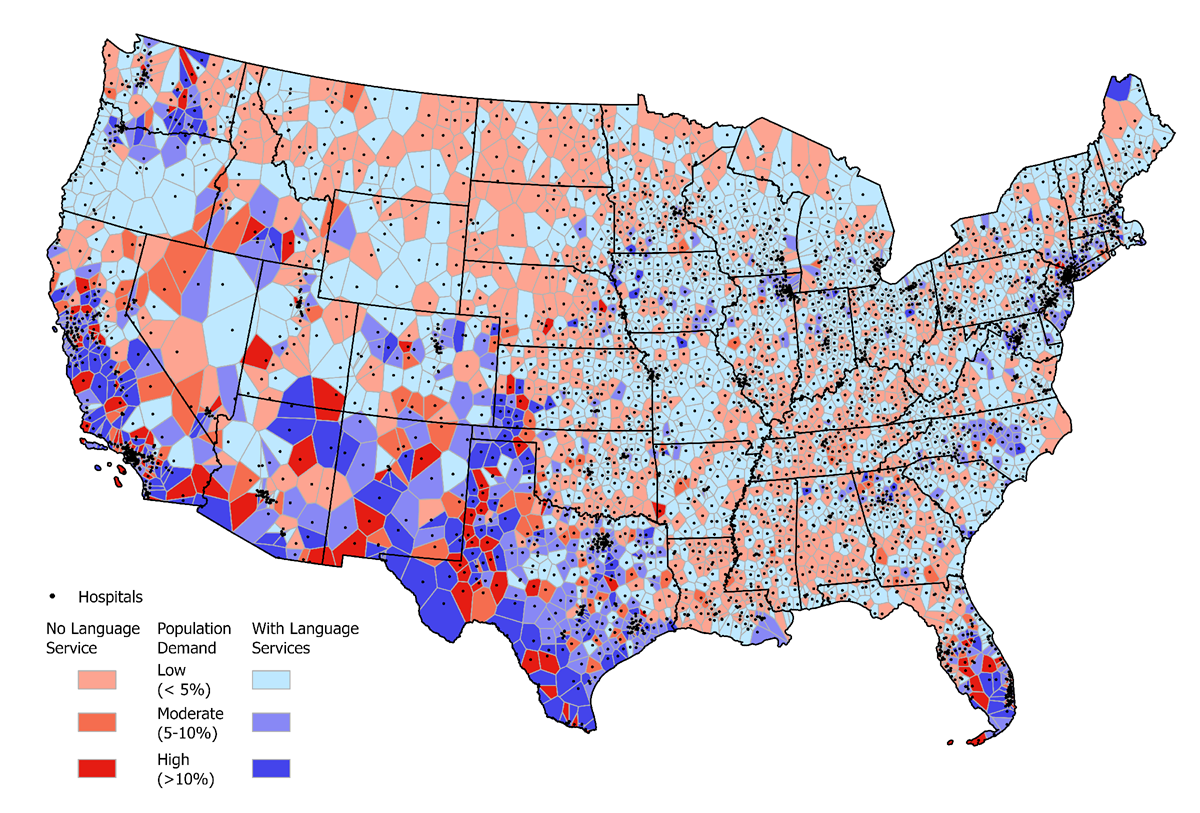
Points and network nodes do not represent areas geometrically, but they can be used to represent areas or contribute to areal operations indirectly, either by storing aggregated areal attributes that summarize individual features within an area or by serving as centers from which areas of influence are derived. For example, city or downtown centroids linked to population data can represent nodal regions, where the point acts as a representative center for a surrounding area or market zone. Similarly, point features such as hospitals or schools can be associated with service or catchment areas derived through network analysis, supporting the delineation of functional regions based on spatial interactions. Techniques such as buffers or Thiessen (Voronoi) polygons enable point features to be transformed into areal representations, allowing the analysis of spatial influence and contributing to area-based analyses. For instance, Schiaffino et al. (2016) applied Thiessen polygons to define hospital service areas by partitioning geographic space based on proximity to each hospital point location, facilitating an assessment of how well language services matched the needs of local populations (Fig. 1).
Line features can represent the boundaries of areas. While lines are useful for delineating the extent or separation of regions, they are limited in areal operations in GIS because they do not represent enclosed space or carry areal attributes on their own. Instead, boundary lines are typically components of polygons, where they form exterior and interior rings that define the geometry and structure of areal features.
Unlike vector-based polygons, which define areas through explicitly drawn boundaries, raster grids represent areas using a regular arrangement of uniformly sized cells. Each cell covers a fixed geographic unit and holds a value for an attribute such as elevation, land cover, or temperature. Areas can be inferred from clusters of contiguous cells with similar values, allowing spatial regions to emerge directly from patterns in the data. This form of representation is particularly effective for modeling continuous spatial phenomena, such as elevation or temperature, where variation occurs gradually and natural boundaries are often diffuse. In such cases, areas may not be defined by external outlines but by the internal structure of the data itself. Raster operations such as region grouping can delineate contiguous patches of similar cell values, identifying homogeneous regions without relying on predefined boundaries. In contrast, operations like zonal statistics summarize raster values within externally defined zones, such as those provided by a categorical raster or a vector polygon layer.
In some cases, geographic areas cannot be easily defined by crisp boundaries due to inherent ambiguity or gradual transitions. Fuzzy areal representation offers an alternative to traditional binary classifications by allowing degrees of membership to a given area that may not have a clearly defined edge (e.g., boundaries between forest and grassland or urban and suburban land use) (Wang & Hall, 1996). Fuzzy logic and fuzzy set theory can be applied in GIS to represent these ambiguous zones, assigning a value between 0 and 1 to indicate the degree of association with a particular class or region. This approach is especially valuable in modeling phenomena with spatial uncertainty or conceptual vagueness, enabling more nuanced areal analysis and decision-making.
Additionally, spatiotemporal representation extends areal modeling by incorporating changes in geographic areas over time (Peuquet, 1994; Yuan, 1996). This is essential for analyzing dynamic areal processes such as urban expansion, deforestation, flood extent, or the spread of disease across regions. In GIS, spatiotemporal data can be represented through time-stamped polygons, time-enabled rasters, or space-time cubes that integrate areal data across temporal intervals. These representations support tracking how areas evolve, merge, fragment, or shift, and enable temporal queries and change detection.
From a fundamental conceptual framework of geographic representation, all geographic information can be reduced to collections of geo-atoms, elemental units of geographic information defined as a tuple <x, Z, z(x)>, where x is a point in space-time, Z identifies a property, and z(x) is the value of that property at that location and time (Goodchild et al., 2007). The various areal representations discussed above can thus be viewed through the geo-atom lens. For example, a polygon may be considered an aggregation of geo-atoms that share the same property value (e.g., land use) across a contiguous area at a particular time.
3. Area Measurements
Measuring the geometric properties of areas is a fundamental operation in GIS, forming the basis for quantifying spatial phenomena and supporting a wide range of spatial analyses. Area refers to the size of a two-dimensional region enclosed by boundaries, while shape metrics describe the geometric form and complexity of that region.
Traditionally, area was estimated using manual techniques such as dot counting, grid cell counting, stripe methods, and the use of polar planimeters. These analog approaches required tracing features or summing overlapping elements over features of interest, and were often tedious, time-consuming, and susceptible to human error. Modern GIS platforms utilize computational algorithms to efficiently and accurately measure the area of digitally represented polygons. Two well-known techniques are the trapezoid method and the shoelace method (Xiao, 2016).
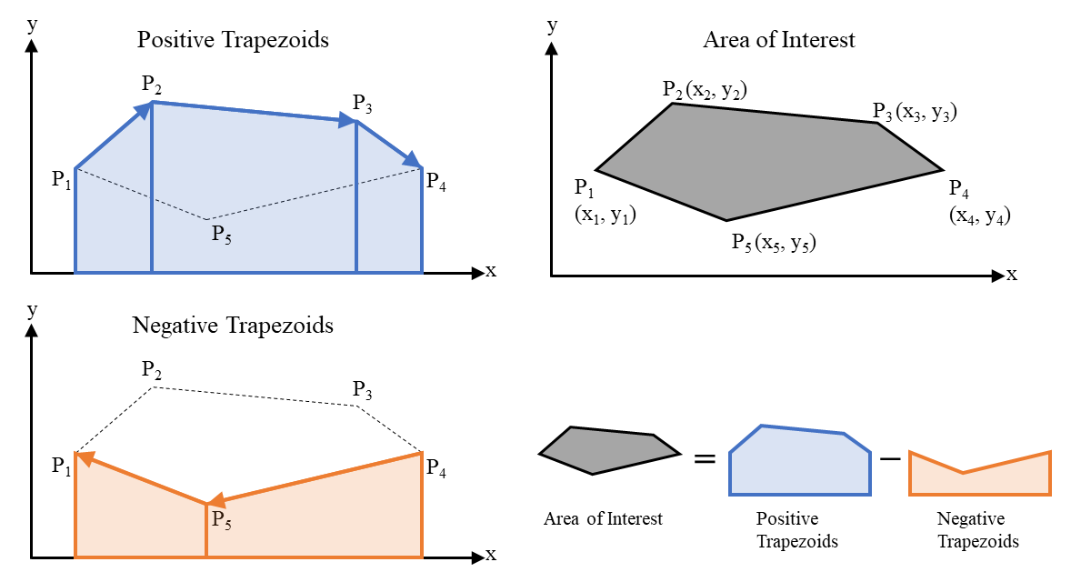
The trapezoid method is a classical technique and conceptually intuitive for calculating area from coordinate measurements. It works by dividing a polygon into trapezoids formed between each edge and the x-axis, then summing their signed areas (Fig. 2). The sign of each trapezoid’s area is determined by the direction of traversal along the x-axis. For each pair of consecutive vertices (xi, yi) and (xi+1, yi+1), the area is positive if xi+1 - xi > 0 (left to right), and negative if xi+1 - xi < 0. By adding the positive trapezoids and subtracting the negative ones, the method cancels out overlapping areas, yielding the correct net enclosed area. The formula for computing the signed area using the trapezoid method is:
where (xi, yi) and (xi+1, yi+1) are the consecutive vertices of the polygon, and n is the number of edges. The polygon must be closed, meaning the first vertex is repeated at the end of the coordinate list.
The shoelace method, also known as the surveyor’s formula, is a well-established technique for calculating the exact area of a closed polygon based on its vertex coordinates. It is particularly efficient for planar polygons represented as a sequence of (𝑥, 𝑦) pairs. The name comes from the crisscross pattern of multiplication that resembles laced shoes. The method computes area by summing the products of coordinates in one direction and subtracting the sum of the products in the reverse direction. The area is calculated using the following formula:
where the polygon is closed by repeating the first vertex at the end. The shoelace method provides a simple, accurate, and computationally efficient approach to handling complex polygon shapes and calculating areas in planar coordinate systems.
Beyond planar calculations, more advanced techniques account for irregular surfaces by incorporating terrain variation. For example, slope-aware area calculations can be performed using Triangulated Irregular Networks (TINs), which model the surface as interconnected triangles. This is particularly important in applications such as hydrology, forestry, and terrain analysis, where surface area differs significantly from horizontal (planar) area due to slope.
Additionally, the choice of map projection significantly impacts area calculations, especially on small-scale maps that cover large geographic extents. Projections such as Mercator or UTM can distort area, particularly at higher latitudes, leading to inaccurate results, while equal-area projections, such as Albers Equal-Area and Lambert Cylindrical Equal-Area, are specifically designed to maintain accurate area relationships. Choosing an appropriate projection is essential for ensuring accurate area measurement, particularly when comparing regions at the continental or global scale.
While area measurement quantifies the size of a region, a range of additional spatial metrics in GIS is used to describe the form, structure, and complexity of areal features. The centroid identifies the geometric center of a polygon and serves as a reference point for spatial joins, distance calculations, and spatial modeling. The perimeter, representing the total length of a polygon’s boundary, is essential for calculating edge-related metrics and plays a foundational role in shape analysis.
A variety of shape measurements have been proposed to assess compactness, which can be used to describe or infer the characteristics of urban form, trade areas, political boundaries, and physical features (Boyce & Clark, 1964). For example, a shape index quantifies the form of an area by measuring its similarity to a standard geometric shape, such as a square or circle, typically through the ratio of the intersection or union between the irregularly shaped feature and the standard shape. Another widely used measure is the compactness index, which can be evaluated based on how efficiently a shape encloses space relative to its perimeter.
Fractal dimension provides a more advanced measure of spatial complexity by analyzing how detail changes with scale. Unlike traditional Euclidean geometry, which defines shapes with integer dimensions (e.g., 1D for lines, 2D for areas), fractal geometry uses non-integer dimensions to reflect how thoroughly a shape fills space. Applied to geographic areas, fractal dimension reveals the irregularity and fragmentation of boundaries across scales, capturing the roughness of spatial forms. It is closely linked to the concepts of self-similarity, repeating patterns across scales, and hierarchy, in which spatial structures are nested. In urban analysis, for example, the fractal dimension of built-up areas can reveal how cities grow in a non-uniform, hierarchical fashion, providing a multi-scalar view of urban growth and sprawl (Batty & Longley, 1994).
4. Areal Operations
Areal operations are fundamental GIS techniques used to analyze spatial patterns, processes, and relationships involving area-based features, which are most commonly represented as polygons. These operations are central to a wide range of applications, including land use planning, environmental monitoring, demographic analysis, resource management, and policy development. By supporting the comparison, aggregation, and interaction of area-based features, areal operations provide essential capabilities for GIS-based analytical reasoning and decision-making.
Table 1 presents examples of polygon-based areal operations across different geometry types, organized by core GIS functionalities. While not exhaustive, it provides a representative range of operations to illustrate the diversity of spatial tasks commonly performed in GIS. Each column includes operations that use polygons as inputs, generate polygons from other geometries (e.g., buffering from points or lines), or involve interactions between polygons and other feature types (e.g., spatial joins with points). Some operations may fall under multiple functional categories depending on the analytical context or software implementation. For example, a spatial join can be classified as an overlay operation, since it links features based on spatial relationships, but it may also serve as an aggregation operation when summarizing information from multiple features. Similarly, Zonal Statistics can be considered both an aggregation method (summarizing raster values by zone) and an overlay (capturing spatial interaction between raster and polygon layers). The table highlights how polygons serve as the dominant spatial framework for organizing, aggregating, and interpreting geographic information across a wide range of analytical contexts. As outlined in Table 1, the following discussion focuses specifically on operations relevant to areal analysis.
Overlay operations combine spatial layers, whether multiple polygon layers or a polygon layer with other geometries, to produce new outputs that retain the spatial and attribute characteristics of each input. Common tools include intersect, union, erase, and identity. As one of the foundational GIS operations, overlay enables the integration of multiple geographic datasets to support further analysis, such as change detection (e.g., identifying land-use change, urban expansion, or deforestation) and suitability modeling, where weighted spatial criteria are combined to inform decision-making (e.g., Weighted Linear Combination, or WLC).
Extraction operations focus on isolating or segmenting features within or based on a polygon boundary. Clip and split are common tools used across vector geometries, while mask is used in raster analysis. These tools help constrain datasets to a region of interest or divide data by administrative or functional zones.
Aggregation operations summarize geometries and/or their attributes within the spatial bounds of polygons, often using spatial joins. Examples include counting crime incidents by neighborhood, calculating the total length of roads in each district, or summarizing service demand from network nodes across cities. Zonal statistics extends this concept to raster data by computing summaries such as mean elevation or Normalized Difference Vegetation Index (NDVI) within each polygon zone.
Generalization operations simplify or restructure spatial data to support more efficient analysis or clearer representation. These include techniques such as dissolve, which merges adjacent polygons with shared attribute values, and others like simplify, minimum bounding box, and convex/concave hull, which reduce geometric complexity or define spatial extents. These techniques are useful for creating regional summaries or generalized boundaries for cartographic visualization and analytical applications.
Proximity operations evaluate spatial relationships based on distance. Buffer creates zones around features to define areas of influence or constraint. Tools such as near and distance matrix calculate distance metrics to or from areal features, typically using the nearest boundary or centroid. Thiessen polygons define regions closest to a point, while network-based service area analysis delineates areas reachable within a specified travel cost or threshold (e.g., distance or time) along a network. These operations are commonly used in service accessibility studies, catchment delineation, and influence mapping.
Validation operations ensure topological correctness and data integrity across spatial datasets. In areal operations, each geometry type may be subject to topological rules in relation to polygons. For polygons, common rules include no overlaps, no gaps, and closed shapes. These validations are essential for maintaining accurate datasets in applications such as cadastral mapping and zoning. Topological rules also apply to points and lines in relation to polygons (e.g., a point must fall within a polygon), as well as to rasters (e.g., a polygon must lie within the raster extent) and networks (e.g., network edges must align with polygon boundaries).
Conversion operations transform one geometry type into another. For example, polygons can be converted to centroids for point-based analysis, to network nodes for modeling accessibility or travel demand, or to rasters for grid-based analysis. These transformations help bridge different spatial data structures in integrated workflows.
Measurement operations use polygons as spatial units to calculate characteristics such as area, perimeter, shape index, and compactness. Other geometry types can also be summarized within polygon boundaries, producing region-based metrics such as point or line density, raster-derived statistics, or aggregated network measures.
While areal operations are an essential part of analytical workflow in many GIS tasks, the implications of MAUP, as mentioned in Section 2, are especially important when combining or comparing data across datasets with different spatial boundaries. To mitigate the impact of MAUP, analysts may adopt techniques such as areal interpolation, which transfers data from one zonal system to another, or dasymetric mapping, which redistributes data using ancillary variables (e.g., land use, impervious surface) to create zones that more accurately reflect the spatial distribution of the underlying variable (Eicher & Brewer, 2001). These approaches aim to align data boundaries more closely with real-world patterns, thereby reducing the bias associated with data aggregation. Additionally, multiscale analysis and sensitivity testing can help assess the robustness of analysis findings to changes in spatial unit definitions.
Table 1. Examples of Polygon-based Areal Operations by GIS Functionality and Involved Geometry Types.
| Functionality | Geometry Type | ||||
|---|---|---|---|---|---|
| Polygon (Single or Multiple) | Line (Single or with Polygon) | Point (Single or with Polygon) | Raster (Single or with Polygon) | Network (Single or with Polygon) | |
| Overlay | Intersect, Union, Symmetric Difference, Erase, Identity, Spatial Join | Intersect, Erase, Identity, Spatial Join | Intersect, Erase, Identity, Spatial Join | Zonal Statistics | Intersect, Erase, Identity, Spatial Join |
| Extract | Clip. Split | Clip, Split | Clip, Split | Mask | Clip, Split |
| Aggregation | Summary Statistics via Spatial Join | Summary Statistics via Spatial Join | Summary Statistics via Spatial Join | Zonal Statistics | Summary Statistics via Spatial Join |
| Generalization | Dissolve, Simplify, Minimum Bounding Box, Convex/Concave Hull | Minimum Bounding Box, Convex/Concave Hull | Minimum Bounding Box, Convex/Concave Hull | -- | -- |
| Proximity | Buffer, Near, Distance Matrix | Buffer, Near, Distance Matrix | Buffer, Near, Distance Matrix, Thiessen Polygons | -- | Service Area |
| Validation | Topology-Rule (e.g., closed, simple, no self-intersection, no overlaps, inside, covered by, intersect, shared boundaries), Eliminate Slivers | Topology-Rule (e.g., inside/covered by polygon, touches polygon boundary) | Topology-Rule (e.g., inside/covered by polygon, not on polygon boundary, each polygon contains at least one point) | Topology-Rule (e.g., polygon must be within raster extent, zones must not be smaller than a cell) | Topology-Rule (e.g., polygon must be served by a connected network, network edges must connect at polygon boundaries) |
| Conversion | -- | Polygon from/to Line | Polygon to Centroid | Polygon from/to Raster | Polygon to Network Node, Constraint Area, or Service Area |
| Measurement | Area, Perimeter, Centroid, Shape Index, Compactness, Fractal Dimension, Area of Overlaps, Length of Shared Boundaries | Line Density per Polygon | Point Density per Polygon | Zonal Statistics describing Polygon (e.g., mean elevation, mean NDVI) | Network Statistics via Spatial Join (e.g., node/line density, connectivity, average travel time per polygon) |
References
- Batty, M. and Longley, P. (1994). Fractal Cities: A Geometry of Form and Function. San Diego, CA and London, UK: Academic Press.
- Boyce, R. R., & Clark, W. A. V. (1964). The Concept of Shape in Geography. Geographical Review, 54(4), 561–572.
- Eicher, C. L., & Brewer, C. A. (2001). Dasymetric mapping and areal interpolation: Implementation and evaluation. Cartography and Geographic Information Science, 28(2), 125-138.
- Gao, S., Janowicz, K., Montello, D.R., Hu, Y., Yang, J-A., McKenzie, G., Ju, Y., Gong, L., Adams, B., and Yan, B. (2017). A data-synthesis-driven method for detecting and extracting vague cognitive regions. International Journal of Geographical Information Science, 31:6, 1245-1271.
- Golledge, R. G. (1992). Do people understand spatial concepts: The case of first-order primitives. In A. U. Frank, I. Campari, & U. Formentini (Eds.), Theories and Methods of Spatio-Temporal Reasoning in Geographic Space (pp. 1–21). Springer.
- Goodchild, M. F., Yuan, M. & Cova, T. J. (2007). Towards a General Theory of Geographic Representation in GIS. International Journal of Geographic Information Science 21(3): 239–260.
- Montello, D. R. (2003). Regions in Geography: Process and Content. In M. Duckham, M. F. Goodchild, & M. Worboys (Eds.), Foundations of Geographic Information Science. CRC Press.
- Openshaw, S. (1984). The Modifiable Areal Unit Problem. Concepts and Techniques in Modern Geography No. 38. Norwich, England: Geo Books, Regency House.
- Peuquet, D. J. (1994). It's about Time: A Conceptual Framework for the Representation of Temporal Dynamics in Geographic Information Systems. Annals of the Association of American Geographers 84 (3): 441–461.
- Schiaffino, M. K., Nara, A., & Mao, L. (2016). Language Services In Hospitals Vary By Ownership And Location. Health Affairs, 35(8), Article 8.
- Wang, F., & Hall, G. B. (1996). Fuzzy representation of geographical boundaries in GIS. International Journal of Geographical Information systems, 10(5), 573-590.
- Xiao, N. (2016). GIS Algorithms. London: SAGE Publications.
- Yuan, M. (1996). Temporal GIS and spatio-temporal modeling. Proceedings of Third International Conference Workshop on Integrating GIS and Environment Modeling, 33.
Learning outcomes
-
1925 - Classify real-world examples of areal features into appropriate region types based on their spatial characteristics and purpose.
Classify real-world examples of areal features into appropriate region types based on their spatial characteristics and purpose.
-
1926 - Identify different ways areal features are represented in GIS, and summarize the strengths and limitations of each representation in various analytical contexts.
Identify different ways areal features are represented in GIS, and summarize the strengths and limitations of each representation in various analytical contexts.
-
1927 - Evaluate the suitability of different area measurement techniques for specific applications, such as land cover estimation, resource management, or urban form analysis.
Evaluate the suitability of different area measurement techniques for specific applications, such as land cover estimation, resource management, or urban form analysis.
-
1928 - Analyze how the choice of areal units can affect the outcomes of overlay and aggregation operations in the context of the Modifiable Areal Unit Problem (MAUP).
Analyze how the choice of areal units can affect the outcomes of overlay and aggregation operations in the context of the Modifiable Areal Unit Problem (MAUP).
-
1929 - Explain how different areal operations modify both geometry and attribute tables, and describe how these outputs differ when working with categorical vs. continuous data.
Explain how different areal operations modify both geometry and attribute tables, and describe how these outputs differ when working with categorical vs. continuous data.
-
1930 - Design a GIS workflow that integrates multiple areal operations to address a complex spatial research question.
Design a GIS workflow that integrates multiple areal operations to address a complex spatial research question.
Related topics
- [AM-02-004] Overlay
- [AM-02-040] Areal Interpolation
- [AM-02-098] Boundaries and Zone Membership
- [AM-03-022] Global Measures of Spatial Association
- [AM-06-102] Volumes and Space-Time Volumes
- [CV-03-004] Scale and Generalization
- [FC-04-040] Neighborhoods
- [FC-05-015] Shape
- [FC-07-026] Problems of Scale and Zoning
- [GS-02-020] Aggregation of Spatial Entities and Legislative Redistricting