[CP-05-031] Apache Hadoop and Spark

Eldawy, A. (2025).  Apache Hadoop and Spark.  The Geographic Information Science & Technology Body of Knowledge (Issue 2, 2025 Edition), John P. Wilson (Ed.). DOI: 10.22224/gistbok/2025.2.22. 

1. Introduction
2. Hadoop vs. Spark
3. Data Model
4. Programming Model
5. Execution Model
6. Structured Queries
7. Conclusion

1. Introduction

MapReduce is a programming paradigm for processing large datasets by dividing work into independent map and reduce tasks. Hadoop’s MapReduce framework pioneered in-situ processing of raw files in a distributed file system (HDFS) without requiring data to be loaded into a traditional database. This was a shift from conventional database management systems (DBMS). Instead of spending hours loading data and creating indexes before analysis, Hadoop can directly scan and process files where they reside on disk. This flexibility comes at the cost of repeatedly reading full datasets for each query and forgoing the query optimizations (like indexes) that DBMSs provide. Still, the MapReduce approach made it feasible to perform analytics over unstructured or loosely structured big data (e.g., massive point clouds or satellite image collections) by leveraging cluster computing for scale and fault tolerance. Traditional DBMSs struggle to scale for such workloads because their strongly typed schemas create significant overhead when ingesting semi-structured data, and their architectures are not optimized for processing massive spatial volumes efficiently.

Both Hadoop and Spark are designed to run on a shared-nothing cluster of commodity machines in a shared-nothing environment, making it relatively simple to set up a cluster. Data files are partitioned into fixed-size blocks (typically 128 MB each in the Hadoop Distributed File System, HDFS), and each machine processes as many local partitions as possible to reduce network I/O. Tasks in these frameworks are stateless and short-lived (often only seconds to a minute each). This design means if a task or node fails, the scheduler can quickly restart that task on another node with minimal overhead, ensuring robust fault tolerance.

In the spatial domain, MapReduce opened the door to “big geodata” processing outside of expensive, specialized database systems. Early efforts simply added spatial operations on top of Hadoop or Spark to utilize their parallel execution, but performance was limited because the frameworks themselves were unaware of geospatial data characteristics. Later, specialized extensions to Hadoop and Spark introduced spatial data types, spatial partitioning, and spatial query optimizations that significantly improved performance for GIS applications. The following sections compare Hadoop and Spark’s core designs and discuss how those designs influence their performance and use for spatial data.

2. Hadoop vs. Spark

While both Hadoop and Spark are big-data systems with many similarities, they have key differences in design and execution:

• Hadoop (MapReduce): Hadoop is primarily a disk-based batch processing engine built around the MapReduce model. A Hadoop job consists of two main user-defined functions, map and reduce, which execute in two stages. First, the map stage partitions the input function and applies the map function in parallel. Second, the reduce phase shuffles the data over network and runs the reduce function to produce the final answer. By default, Hadoop writes all intermediate data to disk between the map and reduce stages to ensure fault tolerance and to minimize memory usage. Complex workflows must be expressed as a series of separate MapReduce jobs, each performing one fundamental step and writing its output to disk before the next step begins. This lack of native support for multi-step optimization means Hadoop jobs are often I/O-intensive and can be harder to develop and maintain when chained together.

• Spark:  Spark, by contrast, is designed as a memory-centric processing engine. It aggressively uses main memory to cache and process data, spilling to disk only when necessary. Spark allows users to define a single logical program that can perform many transformation steps (map-like and reduce-like operations) in one unified pipeline. Under the hood, Spark builds a directed acyclic graph (DAG) of all the operations in the job. This global view gives Spark an opportunity to optimize across the entire chain of transformations, rather than treating each step in isolation. Spark avoids unnecessary disk I/O by keeping intermediate data in memory whenever possible, and it only writes to disk for fault tolerance (checkpointing) or if data does not fit in main memory. The result is often much faster performance, especially for iterative algorithms or multi-stage analytics, since data can be reused from memory across steps. Spark’s ability to combine operations also makes programs more concise and easier to maintain.

In summary, Hadoop follows a pessimistic approach that minimizes memory usage and assumes frequent failures. Spark follows an optimistic approach which assumes abundance of memory and only a few failures. Spark’s assumptions better utilize modern hardware and allows it to scale way beyond Hadoop. However, this comes at the cost of requiring substantially more system RAM on worker nodes to keep datasets in memory and achieve the desired performance.

3. Data Model

Both Hadoop and Spark use partitioned datasets as the core data model. A large dataset is treated as a collection of records (which could be tuples, points, etc.), split into partitions that can be processed independently in parallel. For example, a file might be split into 128 MB chunks that correspond to partitions processed on different nodes. This partitioned model is fundamental to achieving parallelism in both systems.

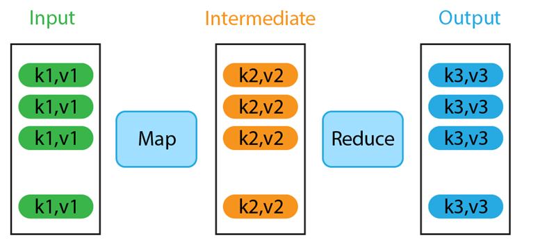
• Hadoop’s data model: In Hadoop MapReduce, a job has three datasets: the input dataset (read from distributed files), the intermediate dataset (the output of the map phase), and the output dataset (the result of the reduce phase, written back to storage). Each dataset is a multiset (bag) of key-value pairs, the keys and values can be of any primitive or user-defined types. Because MapReduce strictly has one map and one reduce stage, there is exactly one intermediate dataset per job. If a program requires multiple processing steps, it must be broken into multiple MapReduce jobs, each with its own fixed input, intermediate, and output sets.
• Spark’s data model:  Spark is more flexible, allowing multiple intermediate datasets within a single application. Spark’s fundamental data abstraction is the Resilient Distributed Dataset (RDD), which represents a distributed collection of records that can be operated on in parallel. RDDs can be created from input files or other RDDs (via transformations) and they persist in memory across stages unless spilled to disk. Spark programs will have an initial RDD (from input data), final RDD(s) for output, and potentially many intermediate RDDs for each transformation in the DAG. RDDs are resilient in that if a partition is lost (e.g., node failure), Spark can recompute that partition by repeating its computation. Like Hadoop’s datasets, RDDs can hold arbitrary records, including spatial objects or key-value pairs. This rich data model makes Spark programs more expressive, as developers can perform complex chains of operations and keep data in memory throughout.

For geospatial (GIS) applications, the records in these datasets typically represent spatial features with geometric attributes (points, lines, polygons, raster tiles, etc.). One common enhancement for spatial data is to apply spatial partitioning, which groups nearby features into the same partition. A simple grid partitioning can be used but highly skewed data require other techniques such as R-tree-based or Quad-tree-based techniques. These techniques build a shallow tree with a few levels on a data sample and use the extents of the leaf nodes as partition boundaries. By partitioning data based on spatial locality, queries can be accelerated: for example, a spatial range query can skip entire partitions that lie completely outside the query window, and spatial joins can be processed mostly within partition boundaries. Both Hadoop-based and Spark-based spatial systems use spatial partitioning techniques to reduce network shuffling and to improve load balancing (ensuring each partition has roughly equal data volume). Partitioning is especially important under the constraints of the MapReduce/DAG models, because minimizing cross-partition communication often means faster and more scalable execution.

4. Programming Model

​​Both Hadoop and Spark rely on a functional programming style, where the computation is expressed as a set of stateless functions applied to data records. A stateless function produces output solely from its input arguments and does not maintain any mutable state between records or tasks. This constraint (a hallmark of functional programming) gives the framework flexibility to parallelize execution and retry tasks safely, if a task is re-run, it will produce the same output since it has no dependence on external state. It also means tasks do not need to coordinate with each other while running, which simplifies distributed execution.

• Hadoop’s model (MapReduce): A MapReduce program in Hadoop consists of two primary functions: map and reduce as illustrated in Figure 1. The user’s overall logic must be mapped into this two-function framework. Simple tasks fit naturally, but more complex algorithms require chaining multiple MapReduce jobs. Each MapReduce job runs independently: after one job produces its output to disk, the next job reads that output as its input. The need to fragment logic into multiple disconnected jobs can make development and debugging cumbersome. For example, implementing a multi-step spatial analysis (like first filtering points by polygon, then joining with another dataset, then aggregating results) would require a series of MapReduce programs with intermediate files, making the workflow harder to manage and slower due to repeated disk I/O.

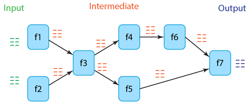
• Spark’s model: Spark generalizes the functional model beyond just map and reduce. It provides a wide array of built-in transformations (e.g., map, filter, groupBy, join, sortBy) and actions (e.g., reduce, collect, count) that developers can combine to express complex logic in a single program. Underneath, Spark takes all these operations and builds a DAG representing the entire job’s logic as shown in Figure 2. This approach has several advantages. First, from a developer’s perspective, the program can be written as one cohesive pipeline, which is easier to understand and maintain than a series of separate scripts. Second, because Spark “sees” the whole DAG, it can perform optimizations across multiple steps. For instance, it can sometimes fuse consecutive transformations into one pass or avoid unnecessary data movement. Third, the operations provided by Spark’s API are highly optimized implementations, often outperforming naive user code. In essence, Spark’s programming model gives the feel of a high-level language with the performance of optimized distributed execution.

For GIS applications, the stateless functional model does introduce challenges. Many spatial algorithms are not trivial to parallelize as map-reduce operations. For instance, building a spatial index (like an R-tree or k-d tree) or performing graph algorithms (like Dijkstra’s shortest path on a road network) typically requires global state or iterative convergence, which doesn’t fit naturally into independent per-record functions. Workarounds often involve breaking such algorithms into smaller functional steps or completely redesigning the algorithm to fit this model. The limitation means that some classic GIS algorithms have to be re-formulated or approximated to run on Hadoop or Spark. For example, instead of constructing an R-tree by inserting records one at a time and updating a shared tree structure, Hadoop and Spark approximate the index using a two-phase strategy. The first phase scans the dataset to extract a representative sample and builds a shallow tree from it. The second phase broadcasts this tree structure and performs a second scan that assigns each record directly to the appropriate leaf partition, which avoids modifying the tree structure as a common state. This is clearly an approximation since it was built on a sample. Other spatial queries (such as range queries, spatial joins, and raster analyses by tiles) can also be expressed in the functional model and benefit from the scalability of these frameworks.

5. Execution  Model

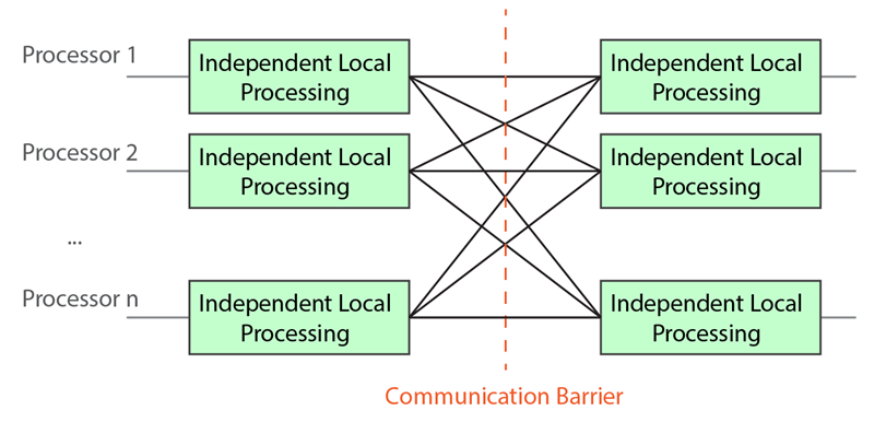
To execute programs in a distributed fashion, Hadoop and Spark both follow a Bulk Synchronous Parallel (BSP) model as shown in Figure 3. In BSP, computation proceeds in discrete stages separated by synchronization barriers. Within a stage, many tasks run in parallel on different data partitions with no communication illustrated as “Independent Local Processing” in Figure 3; when all tasks in a stage finish, the system redistributes data as needed (communication phase) before the next stage begins. This separation of computation and communication simplifies parallel execution because tasks don’t need to coordinate with each other at runtime. Any required data exchange happens in the well-defined barriers between stages.

• Hadoop’s execution: With the MapReduce model, the execution pattern is fixed: a MapReduce job always has two computation stages (the map stage and the reduce stage) and one communication stage in between (the shuffle, which routes intermediate key-value pairs from mappers to the appropriate reducers over the network). This rigid execution model makes Hadoop programs predictable but also somewhat inflexible and costly since each MapReduce job works independently.
• Spark’s execution: Spark must take an arbitrary DAG of operations and map it into BSP stages. It does this by analyzing dependencies between RDDs and classifying them into narrow and wide dependencies. Narrow dependency is a kind of one-to-one dependency that does not require communication between processors. Wide dependency is more general that involves data exchange among all processors, hence, requires a communication barrier. Spark groups together as many narrow transformations as possible into one stage to save network overhead. In effect, Spark’s scheduler slices the DAG into a sequence of MapReduce-like stages automatically. Unlike Hadoop, the number of stages and their boundaries depend on the actual operations used in the program. Many simple Spark jobs end up executing in one stage or a few stages, whereas an equivalent logic in Hadoop might have required more jobs. By managing the execution at the DAG level, Spark can also schedule tasks more efficiently and keep data in memory between stages.

The BSP model in both systems provides the crucial property of fault tolerance: because each stage’s tasks are deterministic and stateless, if a task fails, it can be rerun without affecting other tasks. Hadoop achieves this by re-running map or reduce tasks using the input data (or intermediate data from disk) as needed. Spark achieves it by recomputing lost RDD partitions using the DAG definition and/or by repeating some computation. This means both Hadoop and Spark can scale to thousands of nodes and handle failures gracefully which is a key requirement for long-running spatial analytics on very large datasets.

These BSP constraints require many spatial algorithms to be reformulated, especially when handling boundary conditions. When data is spatially partitioned, algorithms often need access to neighboring features that may reside on another processor, something traditional shared-memory or message-passing approaches allow, but BSP explicitly forbids. In Hadoop and Spark, this challenge is typically addressed in two ways: (1) replicating boundary features into adjacent partitions to avoid cross-partition communication, or (2) deferring boundary records to a later stage where they can be consolidated into a single partition for correct processing.

6. Structured Queries

Originally, Hadoop and Spark were used by writing code (Java, Python, Scala, etc.) to express the data processing. However, many users in both enterprise and research communities prefer using declarative queries (such as SQL) for data analysis. Over time, both ecosystems introduced higher-level query interfaces on top of the core engines:

• In the Hadoop ecosystem, the most prominent query layers were Apache Hive, which runs SQL-like queries, and Apache Pig, which introduces the new Pig Latin language. These allowed users to query data stored in HDFS (e.g., in CSV, JSON, or other formats) without writing MapReduce code directly. The trade-off was that Hive/Pig had to optimize and translate queries into one or multiple MapReduce stages, which added overhead, but they made Hadoop much more accessible to analysts familiar with SQL.
• In Spark, a similar evolution occurred with Spark SQL and the DataFrame/Dataset API. Spark SQL lets users express queries in SQL or via DataFrame operations (which are akin to tables and SQL operations in a programming API). Spark’s SQL engine then plans and optimizes these queries, often achieving better performance than hand-written RDD code because the query optimizer can rearrange and combine operations and push filters down, etc. The DataFrame API provides type-safe, expressive data manipulation without having to drop down to RDDs, and it integrates with Python (PySpark), R (SparkR), and Scala/Java.

For spatial data, these structured query layers have been extended by implementing OGC (Open Geospatial Consortium) standard data types (such as POINT, LINESTRING, POLYGON) and functions (like ST_Contains, ST_Within, ST_Intersection) in their query languages. For example, SpatialHadoop’s Pigeon language extended Pig Latin with spatial data types and functions, and Apache Sedona extends SparkSQL with a catalog of GIS functions. By following OGC standards, these frameworks ensure compatibility with other GIS tools (e.g., one can use the same queries as in PostGIS or Oracle Spatial). This integration means a user can write a SQL query to perform a spatial join or compute an aggregate on spatial data, and the underlying engine will utilize the distributed processing and spatial indexes/partitioning to execute it. The move toward structured queries is part of a broader trend to make big data analytics (including geospatial analytics) more accessible and declarative, rather than requiring low-level programming for every task.

7. Conclusion

Hadoop and Spark have enabled scalable geospatial data processing, with Hadoop offering robust disk-based processing and Spark providing faster, memory-centric execution. Extensions like SpatialHadoop, Sedona, and Beast have added spatial awareness including spatial partitioning, query processing, visualization, and high-level programming languages. As tools improve and integrate structured queries and user-friendly interfaces, big spatial data analytics is becoming more accessible and powerful across the GIS community.

Looking forward, emerging architectures such as GPUs and serverless computing are becoming increasingly prevalent, offering massive parallelism and elastic scalability. Although their potential for spatial workloads is still largely untapped, many of the techniques developed for Hadoop and Spark, such as spatial partitioning and distributed query processing, can be adapted to these new environments to unlock even greater performance and flexibility.

1. Dean, J., and Ghemawat, S. (2008). MapReduce: Simplified Data Processing on Large Clusters. Communications of the ACM, 51:107—113.  https://doi.org/10.1145/1327452.1327492
2. Zaharia, M., Chowdhury, M., Das, T., Dave, A., Ma, J., McCauley, M., Franklin, M. J., Shenker, S., and Stoica, I. (2012). Resilient distributed datasets: a fault-tolerant abstraction for in-memory cluster computing. In Proceedings of the 9th USENIX conference on Networked Systems Design and Implementation (NSDI'12). USENIX Association, USA, 2. https://dl.acm.org/doi/10.5555/2228298.2228301
3. Eldawy, A., and Mokbel, M. F. (2015). SpatialHadoop: A MapReduce Framework for Spatial Data. In Proceedings of the 2015 IEEE 31st International Conference on Data Engineering, Seoul, Korea (South), 2015, pp. 1352-1363. https://doi.org/10.1109/ICDE.2015.7113382
4. Yu, J., Wu, J., and Sarwat, M. (2015). GeoSpark: a cluster computing framework for processing large-scale spatial data. In Proceedings of the 23rd SIGSPATIAL International Conference on Advances in Geographic Information Systems (SIGSPATIAL '15). Association for Computing Machinery, New York, NY, USA, Article 70, 1–4.  https://doi.org/10.1145/2820783.2820860