[DC-02-003] Global Navigation Satellite Systems

Hodgson, M. (2025). Global Navigation Satellite Systems. The Geographic Information Science and Technology Body of Knowledge (Issue 2, 2025 Edition), John P. Wilson (Ed.). DOI: 10.22224/gistbok/2025.2.12.

Acknowledgements

The author expresses appreciation for the review and contributions from Drs. Silvia Elena Piovan and Bruce A. Davis and the anonymous reviewers.

1. Overview
2. Fundamental Advantages of GNSS
3. Determining Position with Trilateration
4. Geometry and Error in the Position
5. GPS Signals
6. Reference Frames
7. The Three Segments of a GNSS
8. Satellite Range Errors
9. Differential GPS
10. Dual Frequency Receiver and Observation
11. Accuracy

1. Overview

The Global Positioning System (GPS) is a satellite-based radionavigation system developed and operated by the U.S. Department of Defense for both the military and civilian communities. The purpose of GPS is to provide users a method for determining accurate positions in 3-dimensional space. GPS is a system composed of three segments: the user, the space, and the control. The user segment refers to GPS receivers in the hands of users or installed in their vehicles, the space segment consists of the constellation of satellites, and the control segment refers to the ground stations that monitor the health of the system. Today, there are over thirty GPS satellites alone at a 20,200 km altitude. Unlike geostationary satellites (e.g. TV broadcasts) the GPS satellites orbit the Earth, each making two revolutions around the Earth every day.

Using GPS accurate positions can be derived using distances from known satellite positions to determine the coordinates of a position on Earth.  The GPS is one of four global satellite-based systems, which are often used concurrently by a “GPS receiver”.   The Globalnaya Navigatsionnaya Sputnikovaya Sistema (GLONASS) is a Russian GNSS. Galileo (named after Galileo Galilei, a polymath scientist) is a European Union system and BeiDou (named after the Big Dipper star constellation) is a Chinese system. All four GNSS have a free and publicly available set of signals called civil signals; additionally, each GNSS has a more encrypted signal for military only use.  While there are some slight differences in some frequencies and data provided, for a fundamental discussion of GNSS we can treat all GNSS as functionally equivalent. Most cellphones today utilize at least two and generally four of the GNSS without the user’s ability to control the specific GNSS used.  For GNSS receivers with improved capabilities the user can, through software apps or even separate controllers, manage the GNSS used, and even the specific signals and other parameters.  For simplicity, much of the discussion below will use the term GNSS and GNSS receiver; however, in a few sections the term GPS is explicitly used when the parameters are unique to the GPS. 

The GPS became fully operational in 1995. The GNSS satellites, their signals, receivers, antennas, and other associated components have and continue to evolve.  This chapter will focus on the fundamental elements which are present today.  The reader should be aware, if looking retrospectively back at historic events, the GNSS environment discussed here may be different than what they find a few years earlier.  This includes terms like the historic use of Selective Availability (to deny all civil users with access to high quality data at a desired time), differential correction (ability to dramatically improve positional accuracy using two receivers), and other changes resulting in improvements in accuracy or availability of satellite signals.

2. Advantages of GNSS

The following advantages of using GNSS over other positioning approaches (e.g. electronic distance based with total station surveying) are notable:

• Global.  As the name implies GNSS is global system offering positioning anywhere on Earth (and somewhat above/beyond Earth). 
• 24/7 Availability.  There are ample satellites now, particularly using all four GNSS, for use any time of the day and any day of the year.
• Free.  Use of the civil signals in all four GNSS is free.
• Weather.  The GNSS signals can be considered all weather in principle although extreme events or even heavy storms can impact the quality of the signals.
• Cost.  To the user, the cost for a GNSS receiver and antenna is very small.  A fundamental unit can be acquired for ~$20 (USD).
• Size.  Compared to many other positioning technologies, the size of the GNSS receiver/antenna is extremely small, with the smallest units only a few centimeters in size, enabling its use in numerous products.
• Passive.  The GNSS receiver only receives radio signals. It does not transmit radio signals (i.e. it is passive) and therefore avoids impacting other nearby radio systems.

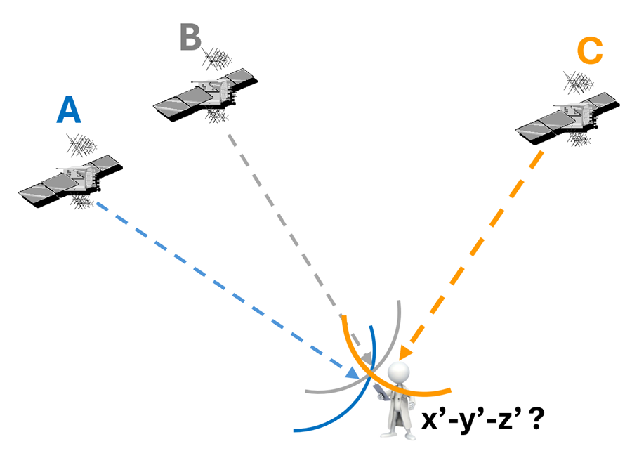
3. Determining Position with Trileration

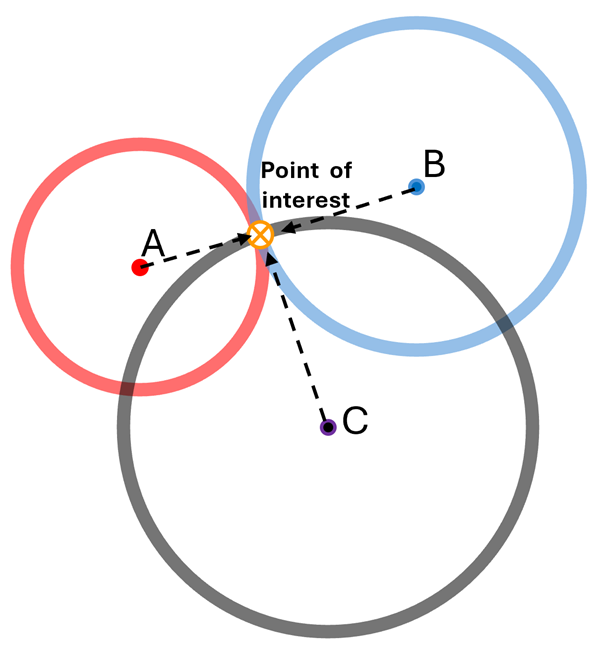
Fundamentally, the GNNS is used to determine the position of a point in 3-dimensional space using the concepts of trilateration (not triangulation) and satellite ranging (Figure 1).  This concept differs from triangulation where both distances and angles from other known points are used.  A position of interest in 2-dimensional space can be precisely determined by knowing the distance of this position from three other points (Figure 2). This concept can be illustrated graphically using circles centered at known points where the radius of each circle is the distance from the known point to the position of interest. The known points could be city centers, towers, church steeples, or survey monuments.  

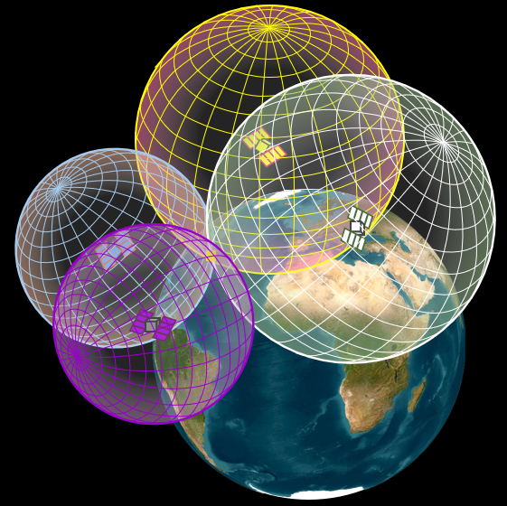
Extending the concept to 3-dimensional space (i.e. the Earth’s surface and circling satellites) requires distances from four satellites and spheres centered at each satellite’s position (Figure 3).  

The distance between satellites and the GNSS receiver is referred to as a range in GNSS literature.  In 3-dimensional space a sphere centered on the satellite’s position is mathematically constructed with a diameter equivalent to the range from the GNSS satellite to the GNSS receiver.   If the range between each of at least four satellites and the receiver is accurately known, the 3-dimensional position of the receiver is determined from the intersection from the spheres (Figure 3).   So, how do we measure range?  If the precise time the signal from a satellite was emitted is known, we can determine range by subtracting emission time from reception time and multiplying by the speed of electromagnetic energy (i.e. ~3x108 m/s).  Thus, the travel time of the satellite signal is a surrogate for the range to the satellite.  Understanding position is fundamentally based on measuring precise travel times of the satellite signals and is key to understanding the sources of travel time errors and how these may be mitigated using additional methods.

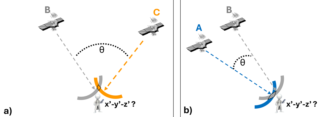
4. Geometry and Error in Position

If the ranges from the receiver to the satellites are determined perfectly, there would be no error in our derived position.  Unfortunately, there are errors in our ranges; thus, the ‘spheres of intersection’ do not intersect precisely at one place (Figure 4a) but result in an intersection of range ‘bands’.  The range band is a sort-of confidence band.  The intersection of the range bands, the geometric configuration of the satellites and their signals used to compute the position influences the accuracy of the position estimate.  As an example, we see the area of intersection is larger with satellites A and B (Figure 4b) than the area of intersection with satellites B and C (Figure 4a). Simply, if the angle formed by emanating lines from the receiver to the two satellites is large the position estimate will be improved.  Historically, with a limited number of satellites and/or constellations, having a good, well-dispersed geometric configuration of satellites was problematic.  Today, particularly using multiple GNSS simultaneously (~136 GNSS satellites of which 35 to 40 are in the user’s horizon), having a good geometric distribution of satellites is not an issue – at least not in an open environment.  When using a GNSS receiver in urban areas or in a mountainous environment where the signals are blocked by buildings or terrain, or even in heavy forested areas where much of the signals are degraded, having a good geometric distribution of satellites can be a problem (Rodriguez-Perez et al, 2007).  Because of the need for a good geometric distribution of satellites the quality of a position is always degraded in these compromised environments.  A good strategy for collecting positions in compromised environments is to take repeat measurements, separated by several hours – if the positions are nearly the same then the confidence in the result is higher.

Finally, the geometric distribution of satellites for terrestrial users of GNSS are always above the horizon (i.e. not below the horizon).  Thus, intersection of the range spheres always results in a better positional accuracy in the horizontal domain than in the vertical domain.  Generally, the vertical accuracy of a GNSS-derived position is about 1.5 to 2.0 times worse than the horizontal position accuracy.

5. GPS Signals

This section describes the names of the GNSS signals, the information carried on the signals, their use in determining satellite to receiver ranges, and the transmission of signals. As of this writing (2025) the satellites of all four GNSS emit signals in three frequencies, all in the radio spectrum L-band. For GPS the signals are referred to as L1 (1575.42 MHz), L2 (1227.60 MHz), and L5 (1176.45 MHz) where the “L” referred to a signal in the L-radio frequency band.  The L1 signal is the primary GPS signal for civilian receivers.  For measurement by wavelength the L1 signal is a 19cm wavelength.  The GLONASS signals are slightly different in frequency and transmit specific data differently.  In comparison, The Galileo signals are called E1, E5, and E6 while the BeiDou signals are B1, B5, and B6.  All three GNSS signals are transmitted from the satellites in the L frequency band, which is effectively free from atmospheric attenuation (e.g. water vapor, carbon dioxide) that would otherwise block the signal transmission.

For GPS, each of the three signals ‘carries’ multiple data streams and thus is sometimes referred to as a “carrier frequency.”  The carrier signal is modulated in a way to carry the coarse acquisition code (i.e. L-C/A code or the more modern L-C code) and navigation data. The C/A or C code data is used for determining the range to the satellite.  The navigation data does not actually transmit the position of the satellite when the signal was generated.  The navigation data includes the ephemeris data that describes the Keplerian motion parameters and the small perturbations caused by the non-uniform Earth gravity field, the sun and moon gravity fields, and atmospheric drag.  With the navigation data and an orbital model running on the GNSS receiver the receiver can predict the location of the satellite at any moment in time, such as the time the signal was emitted.  The navigation signal for each satellite also includes elementary information about the location/ephemerals of the other satellites in the constellation – collectively referred to as the almanac.  The GNSS receiver uses this almanac to initially estimate what satellites should be above the horizon and approximately where each satellite should be at that moment.   Since the almanac must be constantly updated, a GNSS receiver that has not been used for some weeks might need to operate for several minutes after turning it on so the receiver can update its almanac and subsequently provide rapid reliable position determinations.

As of 2025 each of these signals (e.g. L1 or L2) has an additional overlain signal (L1 and L1C, L2 and L2C), but slightly offset.  The advantage of this second signal is a considerable improvement in identifying signals that are reflected from objects on their route to the receiver – a multi-path signal.  Beyond the scope of this discussion are ‘military’ signals (i.e. P and M) that are only interpretable with ‘military’ GPS receivers.

It is important to note the limitations in the GNSS signals.  First, the signals do not pass through solid objects with hardened materials, such building walls, automobile roofs, and thus, are non-functional inside caves and generally inside any structure.  Although the GNSS signals can pass through most windows, the newer high-efficiency windows contain microscopic particles of metal and greatly inhibit the GNSS signals.   Also, the GNSS signals do not penetrate water surfaces, so underwater use is not possible (or not directly possible without a surface antenna).

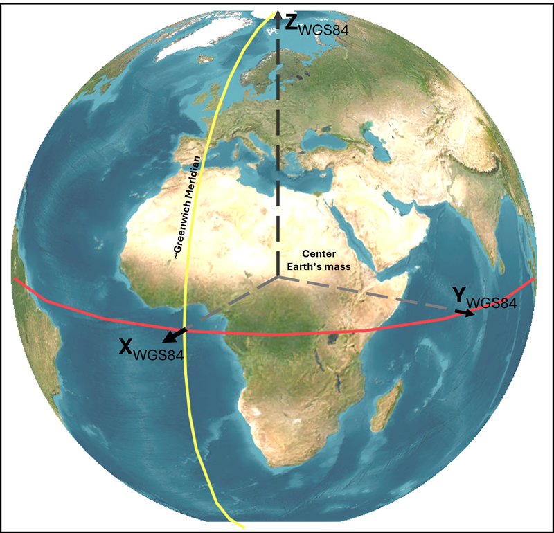
6. Reference Frames

In this section is the discussion of 3-dimensional reference systems for a GNSS, why the reference systems change over time, and their naming conventions.  The 3-dimensional space is a cartesian system where the origin is at the center of the Earth and referred to as an Earth Centered Earth Fixed (ECEF) reference system (Figure 5).   Unlike most datums used for mapping (e.g. NAD83) the ECEF reference system is not directly tied to a continental plate (which constantly move).  And there are many ECEF systems.  For GPS the ECEF system is commonly referred to as the World Geodetic System of 1984 (WGS84), since the ECEF system was originally referenced to the Earth’s parameters (e.g. size/shape, gravity and magnetic fields) as we knew them in 1984. Since the measurements for the Earth’s parameter estimates have improved and the gravity/magnetic fields do change, the realization for the WGS84 ECEF reference system also changes (a bit) over time. The term “realization” refers to the Earth’s known parameters at a specific time, such as the latest version, WGS84(G2296), published in January 2024. (Of note, WGS84 uses the IERS reference meridian which is 5.3 arc seconds east of the historic Greenwich meridian.)  The 2269 refers to the number of weeks since January 6, 1980.  A GPS receiver always uses the latest WGS84 realization.  If a user desires the coordinates to be in a previous WGS84 realization they must transform the positions using software.  Historic collections with GPS may not be important as the changes are typically submeter.  Depending on the application (e.g. surveying, continental motions related to earthquakes), a consideration of the realization used by the GPS at different times is essential.

Other important reference systems use a slightly different naming convention.  As noted above, the WGS84 includes a number for the weeks since January 6, 1980.  Other closely related ECEF systems, such as the International Terrestrial Reference Frame (ITRF) use a designation with the year of the realization and refer to the realization as an epoch, such as ITRF2008 epoch 2005.0 (IERS, 2025). (“Realization” and “epoch” are synonymous.) The WGS84(G2296) aligns with the ITRF2020 epoch. 

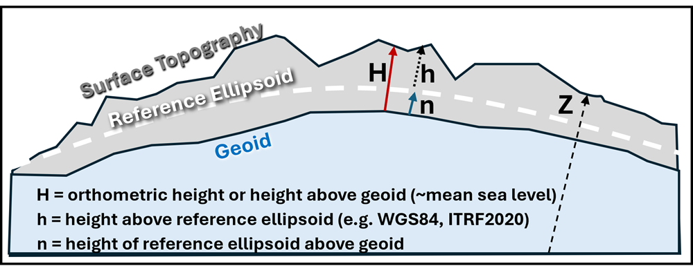
So fundamentally, the GNSS process determines position on the WGS84 ECEF reference frame which is not the reference frame most users need.  However, the ECEF coordinates can be automatically converted to a chosen reference frame (e.g. NAD83, ITRF2014) with the software (e.g. the cellphone native app to iOS or Android, SW Maps) managing the GNSS receiver or GIS software.  The common overlooked part of this process is to recognize the native Z-values from the GNSS receiver are either distances from the center of the Earth (Z), or altitudes above the WGS84 ellipsoid (h), while most mapping scientists are interested in elevation above mean sea level (H) (Figure 6).  Elevation above mean sea level requires a model for where sea level is, even away from the coast.  These elevation models are referred to as geoids.   The difference between height above the reference ellipsoid (h) and elevation defined by the North American Vertical Datum of 1988 (NAVD88) can be up to 36 meters.  Thus, it is imperative to also specify both the horizontal datum (e.g. NAD83) and the vertical datum, such as NAVD88 or the new National Spatial Reference System (NSRS) desired by the managing software.

Finally, the reported time by the GNSS receiver (i.e.  GPS time) is natively related to but not identical to coordinated universal time (UTC) time.  The differences are in seconds and do change every few years.  If precision in seconds is desired the user must compensate for the 18 seconds difference (in 2025) between GPS time and local time.

7. The Three Segments of a GNSS

As noted earlier, there are three segments in the global navigation satellite system.  Of course, the space segment includes the satellites in their orbit around the Earth twice daily (Figure 7).  In the GPS there are 31 operational satellites today.  The number of operational satellites for all four constellations change as satellites are retired and new improved versions are placed in orbit.  The location and trajectory of each satellite (i.e. ephemerals) is determined through ground stations in the control segment that track each satellite. The ground stations located around the world also monitor the overall health of the satellite atomic clocks.  This information is periodically uploaded to each satellite for subsequent transmission in the GNSS signal to the user.

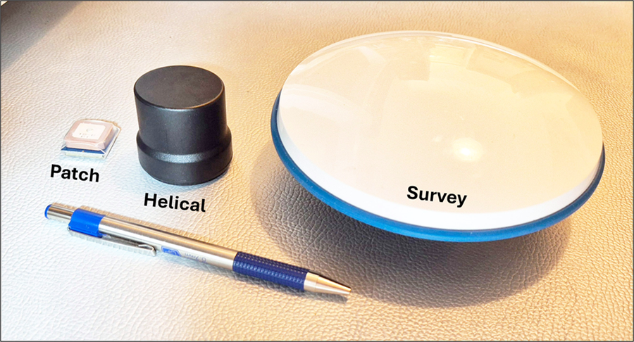
The user segment includes the GNSS receiver, antenna, battery, software, etc. to receive signals and determine positions.  Of note is the common GNSS receiver in a cell phone, relying only on the L1 signal, is very small and has a small antenna (Figure 8).  For improved accuracies with the use of both L1 and L2 signals the antenna is physically larger.  For high-precision applications needing millimeter accuracy the antenna is the largest, well-calibrated, and somewhat expensive.  The recent trend for applications needing sub-meter to centimeter accuracies is using helical antennas which are quite compact.

8. Satellite Range Errors

In this section the primary sources of errors in the positioning process are presented.  Additionally, the statistical terms for characterizing error in a satellite configuration are presented.  GPS satellites today broadcast ranging information in three frequencies, referred to as L1, L2, and L5. The less expensive and simple GPS receivers only use the L1 frequency and are the least accurate in determining positions.  Practically all cell phones, for example, have a GNSS receiver that only uses the L1 frequency.  Spatial accuracies in the best environment are about 3-meters (horizontal) and about 6-meters (vertical).  Improving the accuracy of simple L1-only receivers or the more modern L1/L2, L1/L5, or even the L1/L2/L5 receivers require an understanding of the sources of error in the process for determining positions.  The “error sources” impact the satellite range measurement, resulting in ranges that may be too large or too small. This under/over range estimates explains the depiction of the ranges in Figures 4 as “bands.”  Since the ranges are known to include errors we refer to the ranges as pseudoranges. The primary error sources are:

• Ionosphere and tropospheric delays
• The reported satellite position
• Satellite clock error
• Multi-path travel for a signal
• Local RFI (man-made or natural)
• Geometric configuration of the satellites used in the solution

Various approaches have been proposed to build an “error budget model” where these major errors can be combined to produce a final estimate of the errors in a solution.  An error budget model is useful to model expected errors for a given assemblage of single errors in a geographic context. Except for the geometric configuration of satellites, the other errors can be treated in a Bayesian additive integration.  The geometric configuration of the satellite signals received during a GNSS use is considered a multiplicative error term and thus, is most important.  Additionally, more episodic are the geomagnetic storm that may degrade signal quality; such storms may be forecasted with Kp indexes (Astafyeva et al, 2014).

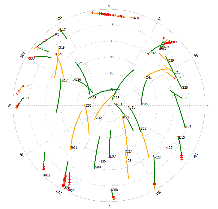
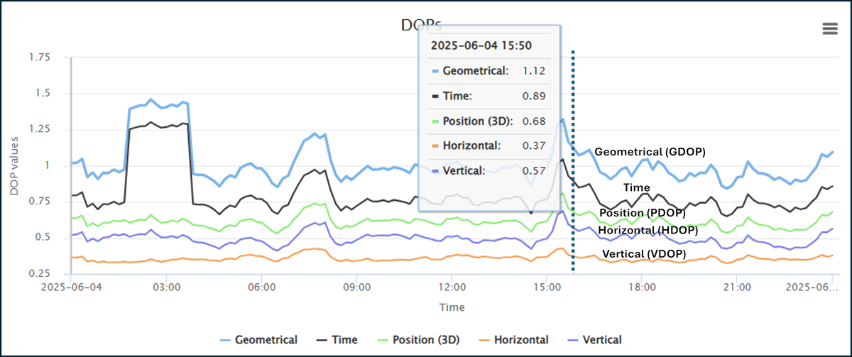
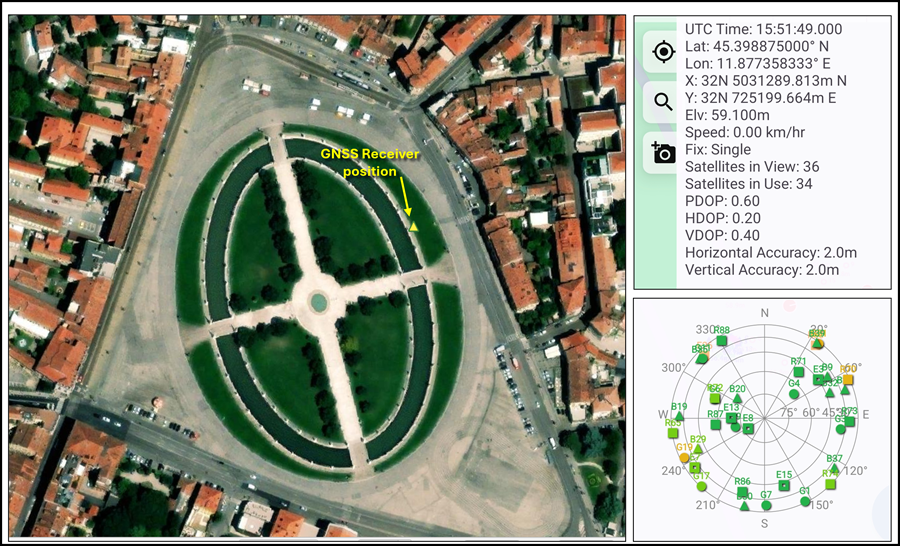
For planning applications needing high accuracy an error budget model is often used.  An error budget model based on the geometry of the satellites (i.e. Figure 4) alone is used by the software (e.g. Trimble Planning in Figure 9) to predict summary error statistics in real-time as the GNSS receiver is operating, such as the Position Dilution of prediction (PDOP), Horizontal Dilution of Precision (HDOP), and Vertical Dilution of Precision (VDOP), shown in Figure 10 using a cellphone-based receiver.  Errors can also be forecasted for a future date based on the satellite constellations at the forecast date/time.  In some applications the user is constrained to only use a limited number of constellations (e.g. only GPS).  For these applications it is useful to forecast the times of the day where the satellite configurations are poor, resulting in lower confidence in position determinations. The user can then avoid collecting data during these periods of time.  PDOP values represent the composite 3-dimensional error and range from a low of 1.0 to over 20.0.  For mapping work PDOP values between 2.0 and 5.0 are considered good; for survey work values less than 2.0 are encouraged.   Predicted PDOP, HDOP, and VDOP for June 18, 2025 (UTC times) are shown in Figure 9 while the actual observed values at the same location at 15:51 UTC are shown in Figure 10.

9. Differential GPS

An early concept for greatly reducing the satellite range errors is to use a second GNSS receiver positioned at a known point and collecting the same observables (e.g. L1) at the same moments in time. The known point might be an existing survey mObserved satellite positions in the hemisphere above a cellphone-based GNSS receiver in the Prato della Valle, Italy on 4 June 2025 in front of the Galileo Galilei statue.  The satellite in view and used in the position fix along with PDOP, HDOP, and VDOP estimates are all very good.onument or a new location whose position is determined with a techniques of higher measurement. This second receiver is called the base receiver while the receiver used to obtain positions at places for which we do not yet have positions is called the rover.  Since the true position of the base is known the true ranges to each satellite can also be known through the application of the Pythagorean formula for the satellite and base positions.  The difference between the true range and the observed pseudorange at the base is called the error. If the rover is ‘near’ (e.g. withing about 60km) to the base the errors observed at the base can be assumed to be the same as the errors experienced (but unknown by the rover) with the rover at each position experiences the same error sources.  This process of using errors determined by a base receiver to correct for the pseudoranges observed at a roving receiver is called the Differential Global Positioning System (DGPS) process.  Without using the DGPS process the positions determined with a roving receiver are often called either stand-alone or single position determinations.  A cell phone GNSS provides single positions determinations.

Two examples are presented where the errors experienced by the base and rover receiver are the same.  The ionosphere and troposphere above the base receiver are effectively the same as these atmospheric constituents above the roving receiver; thus, the satellite signals attenuations are essentially the same. If the satellite clock has an error, then the error is constant for the base and rover receiver.  The observed error at the base is called a correction when used to correct the pseudorange observed at the rover receiver. The greater the distance between the base and rover the greater likelihood the atmosphere the satellite signals travel through will be different and the corrections are not as good.  Remember this degradation of corrections when selecting base receiver data from either free or paid sources of correction data. The utilization of corrections applied to a roving receiver’s observations can be conducted in either real-time or later in a post-processing operation.  In the post-processing process the raw pseudoranges must be logged by the receiver in a file that is later used with a separate data file of corrections from a nearby base receiver.  Thus, the receiver/software used must be capable of logging the pseudorange data.  A number of cellphone apps can be used to accomplish this process.

Another common name for the DGPS process conducted in real-time is called augmentation.  Most large airports have base GNSS receivers operating and producing corrections for the incoming and outgoing aircraft, enabling positional observations with very low errors.  The corrections from the airport receivers are transmitted in real-time via VHF frequencies to the GNSS receivers (i.e.  the ‘rover’ onboard aircraft).  For continental scale applications, satellite-based distribution of corrections is broadcast over an entire continent where the errors are observed at a set of base receivers spatially distributed over the continent.  In the USA this DGPS method of distributing and utilizing the corrections is called wide area augmentation system (WAAS).   In Europe the corresponding system is called the European Geostationary Navigation Overlay Service (EGNOS).  Most cell phones today can utilize WAAS or EGNOS (depending on the phone’s location).  

10. Dual-Frequency Receivers and Observation

Other than the geometric configuration of satellites, the next largest source of error in GNSS receiver use is due to the attenuation caused by the ionosphere and troposphere.  While a GNSS receiver has an estimate of what the signal attenuation might be, the actual attenuation varies from the estimate as the ionosphere/troposphere densities vary spatially and temporally, particularly from storm events.  The common method for obtaining better estimates of the ionospheric delay is to use two frequencies of satellite range estimates, typically L1 and L2.  GNSS receivers using both L1 and L2 signals are commonly referred to as dual frequency receivers.  The L1 satellite signal has a different delay than the L2 satellite signal.  Thus, this measured difference in a delay can be used to effectively remove the ionospheric delay in the signal travel time.  Unfortunately, tropospheric delays do not vary between L1 and L2 signals.  Thus, the difference in expected versus observed tropospheric delays cannot be determined and removed using a dual-frequency receiver independently of augmentation, such as DGPS.

11. Accuracy

11.1 Positional Accuracy

GNSS receivers are used to determine the latitude-longitude-altitude position of the GNSS antenna.  (Not discussed here but the GNSS can also be used to determine very accurate time and velocity.)  In this section, the statistical interpretation of positional accuracy in the GNSS discipline and applications is briefly explained.  Each time a GNSS receiver is used to determine a position the actual latitude-longitude-altitude values will vary, such as 1- to 20-cm or so with L1-only receivers.  The fundamental reason for this is the combination of satellites and their locations have changed since the previous position determination. Remember, the satellites are in constant motion. Repeated position determinations at a known location will use different satellite geometries and possibly different satellite combinations, resulting in slightly different computed positions.  This change in position is temporally correlated with each subsequent position slightly different than the previous.  If mapped, the temporal sequence of observations will follow a path transitioning around the true position.  Expected accuracy can be obtained by collecting a large number of observations at a known point and comparing the computed positions to the known position.  A common statistical summary statistic represents the expected departure from the truth for 95% of all observations collected.  For example, a user of a cellphone based GNSS receiver might expect 95% of the observations collected in obstruction free environments would be within about 3.0 meters of the true location. This 95% accuracy statistic is referred to as Accuracy or Accuracyz if only referring to the altitude errors.  A 68% accuracy statistic is the well-known root mean squared error (RMSE).  Degradation of accuracy using any GNSS receiver is expected in forested environments (Lee, et al. 2023).

However, for a general estimate of the performance of GNSS receivers in the horizontal coordinates (i.e. X-Y) think about 3.00-m, 0.80-m and 0.01-m accuracies at the 95% confidence level for cellphone receivers, L1/L2 receivers in DGPS mode, and receivers using RTK, respectively.  These estimates are based on the assumption of generally clear horizons and definitely not in urban canyons, mountainous terrain, or forested environments (Lee et al, 2023) but vary by leaf-out conditions or canopy closure (Sigrist, 2010; Tomaštík, 2016).

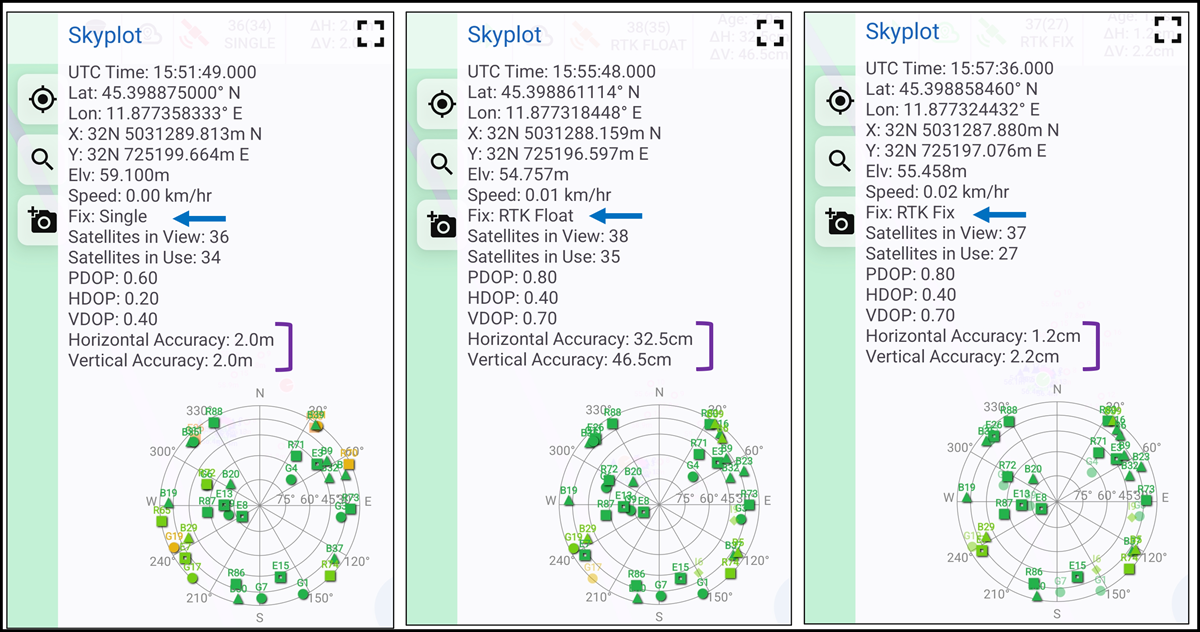
Computation of accuracy is beyond this chapter but is mathematically as simple as the standard deviation formula in slightly altered form.   The common terms used today to describe the quality (actually precision/accuracy) of a geographic position from GNSS use are single, DGPS, float, or fix. The GNSS receiver software reports positions with these terms. “Single” category positions are based solely on the L1 signals from one or more satellite constellations and typically have accuracies in the 2 to 10 meter range (Figure  11).   “DGPS” positions typically result in positional errors of about 1.0m.  “Float” positions have accuracies approximately in the .20 to 1.0 meter range.  “Fix” positions exhibit the highest accuracies of about 0.01-m to 0.03-m (Figure 11).

11.2 Sub-Meter Positioning Accuracy

The fundamental GNSS signal acquisition, processing, and augmentation with the L1 signal typically results in positional accuracies over 1.0 meter. There are approaches for consistently reaching sub-meter and even centimeter accuracies that involave augmentation with dual-frequency receivers and more complex analysis of the signals. Processing approaches suah as real-time kinematic (RTK), post-processing kinematic (PPK), and precice point positioning (PPP) are widely used now by scientists and practitioners. To reach submeter accuracies the use of L1 and L2 signals is essentially mandatory. Moreover, the use of a base and rover receiver is aso required unless the GNSS receiver logs the raw navigation data from the receiver over long periods of time (of least hours of data).  The GNSS receivers and antenna are more expensive, and the antennas are larger (see Figure 8).  A decade ago, the common RTK processing approach required $15,000 (USD) receivers, separate controllers for the software, and often paid subscription services for the augmentation. Today, such receivers for RDK are as low as $150 (USD), the software runs on a user's cellphone, many free augmentation services are available, and the performance is functionally equivalent to the more expensive units (Hodgson 2020).

Official websites for the GNSS:

• GPS: The global positioning system. (n.d.), retrieved on June 30, 2025, https://www.gps.gov/
• GLONASS application consumer center. (n.d.), retrieved on June 30, 2025, https://glonass-iac.ru
• European Union Agency for the Space Programme, European GNSS Service Center (n.d.), retrieved on June 30, 2025,  https://www.gsc-europa.eu/galileo/what-is-galileo
• Chinese government site for BeiDou (n.d.), retrieved on June 30, 2025, https://beidou.gov.cn

Planning Software and Web References:

• Ardusimple (n.d.). “RTK Correction services in your country”, retrieved on June 30, 2025, https://www.ardusimple.com/rtk-correction-services-in-your-country/?mc_cid=e65492c504&mc_eid=560ab0b791
• Planetary Kp-Index (n.d.), retrieved on June 30, 2025, https://www.swpc.noaa.gov/products/planetary-k-index, retrieved on June 30, 2025,
• Trimble GNSS Planning Online (n.d.), retrieved on June 30, 2025,  https://www.gnssplanning.com/#/settings

References

- Abdullah, Q. (2023). The ASPRS Positional Accuracy Standards, Edition 2: The Geospatial Mapping Industry Guide to Best Practices, Photogrammetric Engineering & Remote Sensing, 89(10): 581-588
- Astafyeva, E., Yasyukevich, Y., Maksikov, A. & Zhivetiev, I. (2014). Geomagnetic storms, super-storms and their impacts on GPS-based navigation systems, Space Weather. 12, 508-512
- Hodgson D.L., and Schroeder R.A. (2002). Dilemmas of Counter-Mapping Community Resources in Tanzania. Development and Change, 33(1), 79-100.
- International Earth Rotation and Reference Systems Service (IERS). (2025, June 30). The International Terrestrial Reference Frame.
- Lee T., Bettinger, P., Merry, K., & Cieszewski, C. (2023). The effects of nearby trees on the positional accuracy of GNSS receivers in a forest environment. PLoS One. Mar 15;18(3):e0283090.
- Rodriguez-Perez, J. R., Alvarez, M.F., and & Sanz-Ablanedo, E. (2007). Assessment of Low-Cost GPS Receiver Accuracy and Precision in Forest Environments. Journal of Surveying Engineering 133(4): 159–167
- Sigrist, P., Coppin, P., & Hermy, M. (1999). Impact of forest canopy on quality and accuracy of GPS measurements. International Journal of Remote Sensing, 20(18), 3595–3610.
- Tomaštík, J., Saloň, S., Piroh, R. (2017). Horizontal accuracy and applicability of smartphone GNSS positioning in forests, Forestry: An International Journal of Forest Research. 90(2), 187–198
Learning outcomes
-
880 - Discuss the relationship of GPS to the Global Satellite Navigation System
Discuss the relationship of GPS to the Global Satellite Navigation System
981 - Explain "selective availability," why it was discontinued in 2000, and what alternatives are available to the U.S. Department of Defense
Explain "selective availability," why it was discontinued in 2000, and what alternatives are available to the U.S. Department of Defense
1198 - Explain the relevance of the concept of trilateration to both GPS positioning and control surveying
Explain the relevance of the concept of trilateration to both GPS positioning and control surveying
1939 - Explain how position is determined in X-Y-Z space using the GNSS approach.
1940 - Describe how L1 and L2 signals vary and contribute to positional accuracy.
1941 - Explain why horizontal positions are almost always more likely to be accurate than the vertical positions obtained via GNSS.
1942 - Explain why GNSS receivers cannot determine position within a cave, underwater, or inside buildings.
Related topics
- [CP-03-012] Location-Based Services
- [DC-05-001] Professional Land Surveying
- [DC-05-002] Land records
- [DC-05-041] Ocean Surveying
Additional resources