[DC-04-014] Feature Extraction from Satellite Imagery
Feature extraction in satellite imagery is fundamental to the goal of gathering timely, large-area geospatial information relevant to GIScience research and beyond. There are two approaches in remote sensing to feature extraction. One approach involves identifying phenomena in imagery to be reduced into map form (typically features such as categories or land surface elements). A second approach is to enhance and extract specific bands of imagery and transform them in order to provide a reduced set of inputs or predictors to a model (e.g., a vegetation index). This section focuses only on the former. Extraction of features is performed using a conceptualization of the study site known as a scene model, and the combination of ground reference information and appropriately chosen satellite data. Features can be represented in maps as discrete pixels, polygons or fuzzy membership surfaces, and machine learning algorithms have emerged as the most reliable and effective approaches to feature extraction in the last decade. There are five key steps to performing effective feature extraction: (1) developing a scene model to determine the appropriate scales of information required for a project; (2) ground reference data collection to support the calibration and validation process; (3) selection of appropriate satellite image data, and this can include ancillary data such as digital elevation models; (4) application of a feature extraction algorithm that can best distinguish the feature(s) of interest from background features and produce a map product that is logically consistent; and (5) assessment of map accuracy using validation data to determine the quality of the product for various uses.
Tags
Author & citation
Rogan, J. (2025). Feature Extraction in Satellite Imagery. The Geographic Information Science & Technology Body of Knowledge (Issue 2, 2025 Version), John P. Wilson (Ed.). DOI: 10.22224/gistbok/2025.2.20
Explanation
- Defining the Remote Sensing Scene Model for Feature Extraction
- Acquisition of Ground Referenc Calibration and Validation Data
- Image Preparation and Input Variable Selection
- Selection of Feature Extraction Algorithm
- Map Accuracy Assessment
1. Defining the Remote Sensing Scene Model for Feature Extraction
There are two approaches in remote sensing to feature extraction. One approach involves identifying phenomena in imagery to be reduced into map form (typically features such as categories or land surface elements). A second approach is to enhance and extract specific bands of imagery and transform them in order to provide a reduced set of inputs or predictors to a model (e.g., a vegetation index). This section focuses only on the former. The key to successful feature extraction is to enhance the feature of interest so it is statistically separable from all other features (e.g., to separate tree canopy cover from roads and shadows). When multiple features are of interest, those features must be statistically separable from one another. The process of feature extraction from satellite imagery involves five important steps. Step 1 requires that a scene model be created for the task (Strahler et al. 1986; Phinn 1998). The scene model defines the feature or features under investigation in terms of their spatial, temporal and spectral dimensions absent any multispectral data. Subsequently, the scene model framework (see Table 1) allows for the careful selection of appropriate satellite data to ensure accurate and efficient feature extraction. An important component of the scene model is the definition of (H)igh versus (L)ow spatial resolution for feature extraction. H-resolution implies that the pixel spatial dimensions are physically smaller than the feature whereas L-resolution implies that the pixel spatial dimensions are larger than an individual feature in the scene. H-resolution is preferable when the application is to finely resolve scene features. However, L-resolution is necessary for global scale analyses and biophysical assessments of water quality, surface temperature and airborne particulate matter.
2. Acquisition of Ground Reference Calibration and Validation Data
The second step in the feature extraction process involves the creation of a database that contains fine-grained information on the location and characteristics of the feature (see Figure 1). A variety of data can be used including in situ field data, historical data, aerial photographs or high-resolution drone aircraft data. In some cases, pseudo-invariant data may be used such as long-term observation sites showing little environmental change over time. Additionally, spectral libraries may also be used if they are representative of the study area under investigation.
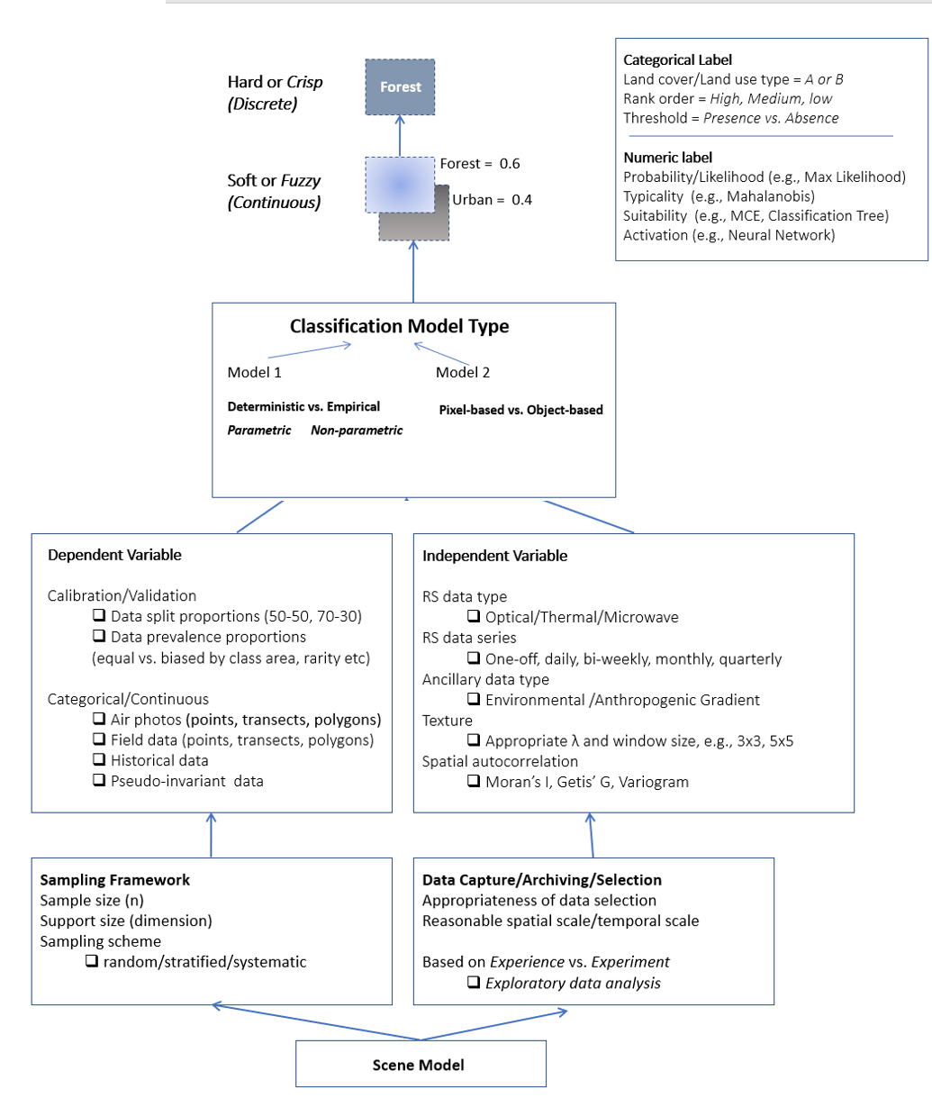
The creation of a ground reference database is also determined by the intended by the classification scheme, or desired map legend. In some cases, only one feature is being mapped (e.g., forest cover), whereas in other cases multiple features are being mapped (e.g., forest, grass, urban and water). Map legends are recommended to be mutually exclusive, exhaustive and hierarchical.
When working with calibration and validation data, the sample size, distribution among features and representativeness play a very important role in the success of the feature extraction process (Muchoney and Strahler 2002). Typically, ground reference data are split proportionally into calibration and validation data sets (e.g., 50:50, 70:30, or 80:20). Machine Learning algorithms typically perform best when provided with a high number of calibration data. In cases where many different types of features are being extracted from satellite data, careful attention should be paid to the landscape distribution and prevalence of particular features in order to represent them appropriately when processing an algorithm. For example, when mapping land cover features in a forested mountainous region, calibration sample size should be biased toward forest features in order to capture the spatial variability and non-stationarity present in the landscape due to the wide geographic expanse and presence of a steep elevational gradient. It is important to note that some remote sensing practitioners advocate for the use of balanced calibration data (i.e., equal number of samples for all categories).
3. Image Preparation and Input Variable Selection
The third step in the feature extraction process is to determine the appropriate satellite data to be employed. Use of the scene model (Table 1) can guide the choice of satellite imagery in terms of three types of resolutions: spatial (pixel size); spectral (wavelengths); and temporal (frequency of acquisition). As shown in Figure 1, there is wide variety of satellite data available ranging from multispectral to thermal, RADAR and LiDAR. Selection of imagery is determined by availability, quality and cost although all three factors have improved considerably over the past 20 years. Satellite data provided by NASA’s Landsat program (30 m resolution, multispectral), and the ESA’s Sentinel-2 program (10 m resolution, multispectral) are free for download and have high spatial and radiometric quality, and are available on Google Earth Engine To date, data with a finer spatial resolution than Sentinel-2 are not freely available, with the exception of the USDA’s National Agriculture Imagery Program (NAIP) which captures 0.3 – 0.6 m spatial resolution, multispectral aerial imagery on a two-year basis and can be downloaded from the NAIP website. Additionally, LiDAR data are freely available from the U.S. Geological Survey’s LiDAR online repository. Fine-grained multispectral imagery such as NAIP can be complemented, at cost, by satellite data from commercial providers such as MAXAR who provide high quality data from their suite of WorldView satellites.
Table 1. Draft scene model specifications for feature extraction from satellite imagery, using adult African elephants as an example of the feature of interest. The process starts with the identification of the specific feature of interest and the environmental characteristics that constrain it. The next step in the process is to identify the spatial, temporal and spectral dimensions of the feature so that selection of satellite imagery will be optimized, if such optimal data are available. The final step is to determine how much error is tolerable in feature labeling.
| List of Specification | Key Questions | Application to Elephant Detection |
|---|---|---|
| Information Required | What is the feature of interest (i.e., response variable)? | Biophysical parameter: Individual African elephants - in contrast to trees, shrubs, water, shadow, bareground, or shadow. |
| Environment Type | What are the typical measurable characteristics of this location? | Broadleaf woodland and shrubland with pronounced dry vs. wet seasons; Extensive area of bare soil and rock. |
| Spatial Scale | What is the finest dimension of the phenomenon of interest, and over what geographical extent? | Grain = Typical body length of acult elephant (305 m); Extent = Chizarira National Park (Zimbabwe): 490,000 acres |
| Temporal Scale | How often do you need to observe the phenomenon, and at a date and time when it is most visibly apparent? | One image per season at the time of maximum spectral separability for individual (adult) elephants |
| Components and Hierarchy | Constraint = Landscape extent? Focus = Scale of detection for the project? Mechanism = Finest physical expression of phenomenon? |
Constraint = Chizarira National Park (Zimbabwe) Focus = Adult elephants Mechanism = Individual elephants of all ages |
| Spatial Dimensions | H vs. L Resolution? Grain = Finest spatial resolution to detect individuals Extent = Area required for image areal coverage |
H-resolution Image Grain = 1-2 m Image Extent = 772 square miles |
| Temporal Dimensions | What is the optimal date(s) ni a year to observe the phenomenon? What is the optimal time of day to observe the phenomenon? What interannual considerations need to be made? |
Optimal Data = April to October (dry season / fewest clouds) Solar conditions = 0-20 degrees solar zenith Interannual = near anniversary dates and acquisition times |
| Spectral Dimension | What are the best wavelengths / spectral band indices to enhance the phenomenon of interest and reduce the influence of background features? | Blue = 380 to 500 nanometers (nm) Green = 495 to 570 nanometers (nm) Red = 620 to 750 nanometers (nm) |
| Error Tolerance | How much error is acceptable in the detection of the phenomemon of interest? | Calf and juvenile elephants are not considered due to their small dimensions Elephant adults detected +/-1 m |
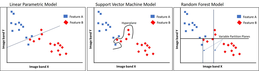
The accuracy and efficiency of feature extraction is often improved through the integration of satellite data representing different portions of the electromagnetic spectrum (e.g., optical, thermal, microwave) as well as enhancements of those data, such as a vegetation index in the case of multispectral data, and a texture transformation the case RADAR imagery. The combination of different types and enhancements of satellite data has been shown to substantially improve the accuracy of map products by increasing the statistical separability of features in a scene (Zhu et al., 2012). Satellite data sets may also be combined with ancillary data sets representing eco-climatic gradients including digital elevation models (DEMs) and socio-economic information such as land tenure and historical land use (Franklin 1995). Ancillary data improve the performance of feature extraction by increasing the dimensionality of the data volume, and by representing sources of non-stationarity across a landscape that may be omitted by using satellite data alone. Machine learning algorithms are particularly well suited to process the large data volumes in integrated data sets. Figure 2 shows a schematic example of the statistical separability in a hypothetical multispectral image data volume. For the data shown in figure 2 the parametric model is incapable of separating overlapping features from different classes, whereas the Support Vector Machine hyperplane and the Random Forest variable partition planes can address this class mixing in different ways.
4. Selection of Feature Extraction Algorithm
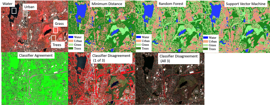
The fourth step in feature extraction process involves the selection of the appropriate algorithm. Those algorithms are traditionally known as ‘classifiers’ although many do not solely perform classification tasks. Figure 1 shows that there are two typologies of feature extraction models. The first type concerns parametric vs. non-parametric approaches. Parametric approaches assume normally distributed satellite data and a thorough understanding of the probability density function of the feature. Examples include supervised maximum likelihood classification and unsupervised clustering (e.g., ISODATA). Parametric approaches were very popular in the 1970s and 1980s but were replaced by the more versatile non-parametric approaches in the 1990s-onward as remote sensing projects became more expansive, complex and demanding. Non-parametric approaches such as artificial neural network algorithms make no assumptions about the satellite data probability density, and rely heavily on the quality of the calibration data set. Figure 3 shows a comparison of three non-parametric algorithms in an urban landscape. The feature categories are urban, water, grass and trees.
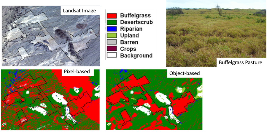
The second model type concerns pixel-based vs. object-based approaches. Pixel-based approaches result in features being labeled on a per-pixel basis with no indication of whether that pixel is part of a feature or the whole feature element, while object-based approaches are derived via segmentation algorithms that delineate features as homogeneous objects, that are subsequently labeled by a non-parametric algorithm. During the last step of any feature labeling process, the output may be fuzzy (soft), or hard (discrete). A fuzzy output represents a continuous value representing probability, typicality or suitability, depending on the particular algorithm. A hard output indicates a categorical label representing a qualitative label, or presence versus absence of a feature in the map product. Choice of fuzzy versus hard labels depends on the goal of the project, but in practice, a ‘hard classification’ is seen by most as a key endpoint in the entire feature extraction workflow. Figure 4 shows a comparison of pixel-based versus object-based classification using Landsat-5 imagery in a semi-arid region depicting a site where an ornamental grass was planted in fenced pastures to boost cattle forage.
Supervised machine learning algorithms are a special type of non-parametric model that learn from calibration data errors during the pixel labeling process and improve their performance without user intervention (unsupervised machine learning algorithms do not require calibration data). There are many types of machine learning algorithms and the choice of implementation is attributed to their accuracy, complexity, transparency, and user familiarity. The K-Nearest Neighbors (KNN) and Support Vector Machines (SVM) are popular supervised algorithms used in image classification and regression. They work by determining how similar unlabeled pixel values are to those in the calibration data, or the theorized subset of calibration data most likely to be confused. Random Forest classification and regression uses recursive partitioning of input variables to determine how unlabeled pixels can be sub-divided into smaller sub-groups of features (Breiman, 2001).
The fifth step in feature extraction is map accuracy assessment with the validation data set described previously. The validation data are used to calculate a variety of metrics to determine the quality of the map product through assessment of prediction errors (Fielding and Bell 1997). The metrics can be used to communicate to map users how appropriate the map is for navigation, planning and follow-up spatial modelling. Additionally, the metrics can be used to re-evaluate the calibration process/output and re-run the algorithm pursue a better outcome.
References
- Breiman, L. (2001). Random Forests. Machine Learning. 45, 5–32.
- Fielding, A. H., & Bell, J. F. (1997). A review of methods for the assessment of prediction errors in conservation presence/absence models. Environmental Conservation, 24(1), 38–49.
- Franklin, J. (1995). Predictive vegetation mapping: geographic modelling of biospatial patterns in relation to environmental gradients. Progress in Physical Geography: Earth and Environment, 19(4), 474-499.
- Muchoney, D.M., and Strahler, A. H. (2002). Pixel- and site-based calibration and validation methods for evaluating supervised classification of remotely sensed data. Remote Sensing of Environment 81(2-3): 290-299.
- Phinn, S. R. (1998). A framework for selecting appropriate remotely sensed data dimensions for environmental monitoring and management. International Journal of Remote Sensing, 19(17), 3457–3463.
- Strahler, A. H., Woodcock, C. E., and Smith, J. A. (1986). On the nature of models in remote sensing. Remote Sensing of Environment 20(2): 121-139.
- Zhu, Z., Woodcock, C. E., Rogan, J., and Kellndorfer, J. (2012). Assessment of spectral, polarimetric, temporal, and spatial dimensions for urban and peri-urban land cover classification using Landsat and SAR data. Remote Sensing of Environment (117): 72-82.
Learning outcomes
-
1990 - Describe the five steps required to perform feature extraction on satellite imagery.
-
1991 - Describe the scene model and its importance in feature extraction.
-
1992 - Explain the different types of ground reference data used in feature extraction.
-
1993 - Differentiate between parametric and non-parametric algorithms, and pixel-based versus object-based feature extraction.
-
1994 - Explain the key differences between commonly used machine learning algorithms used in feature extraction.
Related topics
Additional resources
- The National Agriculture Imagery Program (NAIP), https://naip-usdaonline.hub.arcgis.com/
- NASA’s Landsat Program, https://landsat.gsfc.nasa.gov/
- The European Space Agency’s Sentinel-2 Program, https://www.esa.int/Applications/Observing_the_Earth/Copernicus/Sentinel-2