[DM-05-048] Planar Coordinate Systems and the U. S. National Grid

Koylu, C., and Chan, C.-H. (2025). Planar Coordinate Systems and the U. S. National Grid. The Geographic Information Science & Technology Body of Knowledge (Issue 2, 2025 Edition), John P. Wilson (ed.).   DOI: 10.22224/gistbok/2025.2.17.

1. What Is a Planar Coordinate System?
2. Planar Coordinates
3. Using a Planar Coordinate System
4. National Grid Systems and The U. S. National Grid

1.  What is a Planar Coordinate System?

A planar (projected) coordinate system (PCS) assigns a unique index to mapped locations on a two-dimensional planar (flat) surface. Unlike a geographic coordinate system (GCS), which overlay a graticule on the curved surface of the Earth as defined by a geodetic datum or ellipsoid, planar systems transform the Earth's three-dimensional shape into a flat plane using a map projection. These systems are critical for detailed calculations and accurate positioning, particularly for large-scale (small area) mapping where accuracy in relative positions is essential.

To create a planar coordinate system, a map projection must first be applied to convert the Earth's surface into two dimensions. The choice of projection significantly influences the accuracy of the resulting map, as all projections introduce some degree of distortion in areas, angles, distances, or directions. For this reason, planar coordinate systems are most commonly used for large-scale mapping at scales of 1:24,000 or larger, where distortions can be minimized within a small geographic area.

To further enhance accuracy, particularly when performing measurements, a projected coordinate system is often divided into smaller zones, each with its own projection parameters and center. This zonal approach helps maintain precision in feature location and positioning relative to other features, even over large areas.

A planar coordinate system is based on a Cartesian grid, where perpendicular x (east-west) and y (north-south) axes define positions on a flat surface. Each grid square represents a unique location, with coordinates assigned to represent east/west and north/south positions. This system provides an intuitive and practical way to calculate distances and areas on a map, but careful consideration must be given to the choice of map projection to balance accuracy and distortion.

The decision on which map projection to use when establishing a planar coordinate system is crucial and involves a trade-off between preserving certain geographic properties, such as shape, area, distance, or direction. Some projections are designed to preserve one or more of these characteristics over small areas, while others are optimized for specific types of analysis. A detailed discussion on the selection of map projections could be explored further in the GIS&T Body of Knowledge article on map projections (Battersby 2017).  

2. Planar Coordinates

In a planar coordinate system, the Earth's curved surface is transformed into a flat plane, and locations are identified using mutually perpendicular axes, typically referred to as the x (east-west) and y (north-south) coordinates. Unlike geographic coordinate system, which retains the spherical or ellipsoidal nature of the Earth, a planar coordinate system is built upon Cartesian coordinates and is used for precise positioning and distance measurements, especially for large-scale maps. The choice of map projection directly influences the accuracy of the x and y coordinates, as different projections handle distortions in size, shape, and distance in varying ways.

Latitude and longitude are angular measurements, which represent positions on the Earth’s surface relative to the center of the Earth. Latitude measures the angle north or south of the equator, while longitude measures the angle east or west of the Prime Meridian. These are expressed in degrees, minutes, and seconds (or decimal degrees), which are inherently related to the curvature of the ellipsoid used to approximate the Earth’s shape.

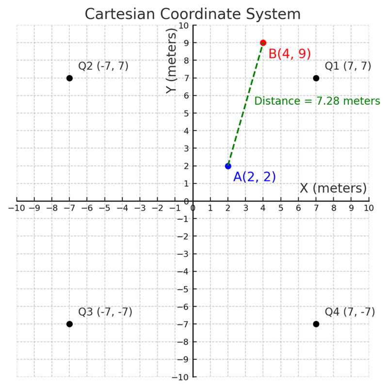
In contrast, Cartesian coordinates (x and y) in a planar coordinate system are linear measurements on a flat, two-dimensional surface. These units represent actual distances from a defined origin, typically at the intersection of perpendicular axes. Unlike angular measurements on a curved Earth surface, such as latitude and longitude, Cartesian coordinates are measured in consistent, standard units like meters or feet. This uniformity simplifies calculations of distance, area, and other spatial properties, making the system highly suitable for practical mapping and analysis. For example, the Euclidean distance between two points, A (2,2) and B (4,9), can be easily calculated using the Pythagorean theorem (Figure 1). The distance is determined by calculating the straight-line distance between the two points along the 𝑥 and 𝑦 axes, which is computed as:

To avoid negative coordinates on a map, map projections employed for planar coordinate systems produces a false origin specified with false easting / false northing values, which offset the true origin of the projection that the ellipsoid and the flat surface coincide. As a result, a planar coordinate system produces coordinates with positive values towards east and north of the origin.

3. Using a Planar Coordinate System

In practice, planar coordinate systems divide large areas into smaller zones, each with its own projection center to minimize distortions. This zoning enables higher positional accuracy within each zone, particularly in measuring the location of features and their spatial relationships. Different projections preserve different spatial properties such as area, shape, distance, or direction to make them suitable for specific mapping and spatial analysis needs.

Common planar coordinate systems include the Universal Transverse Mercator (UTM), the State Plane Coordinate System (SPCS), and the Lambert Conformal Conic (LCC). The LCC projection, for example, is a secant conic projection that preserves shape (conformality) and is particularly well-suited for mapping mid-latitude regions that extend more in the east-west direction. It is widely used in North America, including for aeronautical charts and in many state plane zones, because it minimizes distortion between its standard parallels.

The choice of an appropriate plane coordinate system depends largely on the spatial extent of the area being mapped and the required positional accuracy. For large-scale, localized projects—e.g., municipal engineering, cadastral surveys, or the construction of infrastructure within a state or county in the United States—the State Plane Coordinate System (SPCS) is generally the most suitable. The zones are intended to reduce distortion in individual states or regions so as to provide sub-meter accuracy for surveying and design. For regional to national scale mapping involving several zones or countries, the Universal Transverse Mercator (UTM) system is used because it has a consistent metric framework and extensive coverage of the globe, providing a reasonable balance between accuracy and convenience. For applications on a global scale or for aviation purposes requiring large spatial coverage and less demanding metric accuracy, systems like the World Geographic Reference System (GEOREF) may be more appropriate. Each system has distinct advantages, and the ideal choice hinges on scale, accuracy requirements, and geographic coverage.

3.1 The Universal Transverse Mercator (UTM) Coordinate System

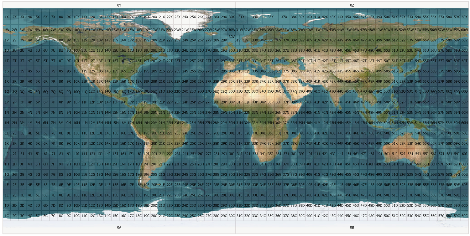
The Universal Transverse Mercator (UTM) Coordinate System is one of the most commonly used coordinate systems worldwide. It provides a global framework for mapping and spatial analysis by dividing the Earth's surface into manageable zones that minimize distortion. The UTM system divides the Earth’s surface into 60 zones, each 6 degrees wide in longitude (Figure 2). These zones are numbered from 1 to 60 in an easterly direction, starting from the International Date Line (180° West longitude. Each UTM zone is further divided into northern and southern hemispheres, indicated by an “N” (North) or “S” (South) designation using the equator as the divider. For example, zones containing most part of Japan are designated UTM Zone 53N and UTM Zone 54N, Ecuador is in UTM Zone 17S, where “S” indicates its position south of the equator.

The datums referenced here—North American Datum of 1927 (NAD 27), North American Datum of 1983 (NAD 83), and World Geodetic System 1984 (WGS 84)—define the mathematical surfaces and coordinate origins used for mapping. NAD 27 is based on the Clarke 1866 ellipsoid and a single U.S. survey control point, whereas NAD 83 and WGS 84 are Earth-centered datums based on global satellite observations. See individual topics within Georeferencing Systems as well as Coordinate Transformations (Seong 2023) for more background.

One thing to keep in mind is that the UTM system covers latitudes from 80°S to 84°N, meaning that the polar regions are not projected using UTM. Instead, another projected coordinate system, the Universal Polar Stereographic (UPS) projection, is used for latitudes beyond 80°S and 84°N.

In the UTM system, locations are specified using UTM Eastings and Northings, which represents distances in meters from the zone’s origin. UTM Eastings (x-values) increases in an easterly direction, while Northings (y-values) increase northward. Each UTM Zone has a central meridian and false easting, and northings are applied to each zone.

The central meridian is assigned a false easting of 500,000 meters to keep all eastings positive. In the southern hemisphere, a false northing of 10,000,000 meters ensures all northing values remain positive. Here, the equator starts at 10,000,000 meters, decreasing toward 0 meters at the South Pole. In addition, it is essential to note that a projected coordinate system includes a datum. UTM coordinates vary depending on the datum used, such as NAD 27, NAD 83, or WGS 84. For example, UTM Zone 15N based on NAD 83 would be designated "NAD 1983 UTM Zone 15N," while the same zone under WGS 84 would be "WGS 1984 UTM Zone 15N." Properly specifying the datum is crucial, as the same UTM coordinates can differ based on the datum applied.

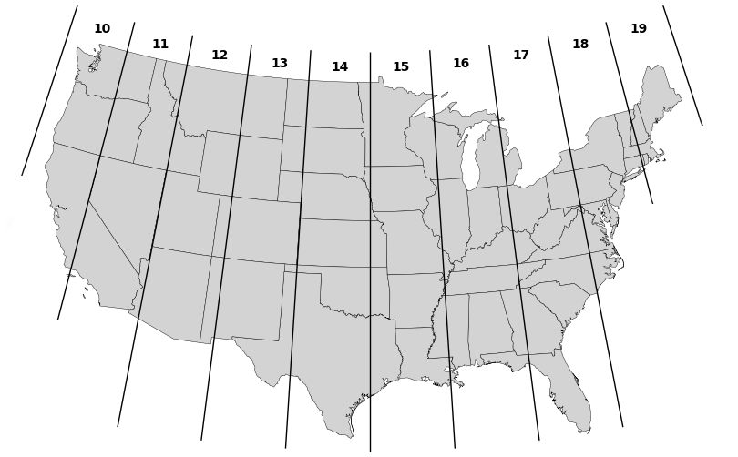
In the United States, UTM zones are particularly useful for mapping and geospatial analysis within a given area limited to a zone up to 6 degrees wide in longitude. The division of zones across the U.S. means that some states fall entirely within a single zone, while others are split between two or more (Figure 3). For instance, states like Alabama and Colorado are mostly contained within a single UTM zone which are16N and 13N respectively. However, states such as California, Texas, and New York span multiple zones due to their east-west extent. California is primarily covered by Zones 10N and 11N, while Texas stretches across Zones 13N, 14N, and 15N. Many state-level agencies distribute spatial data in UTM coordinates because a state often falls entirely or predominantly within one UTM zone, making data management and analysis more straightforward and easier.
 

3.2 The State Plane Coordinate System

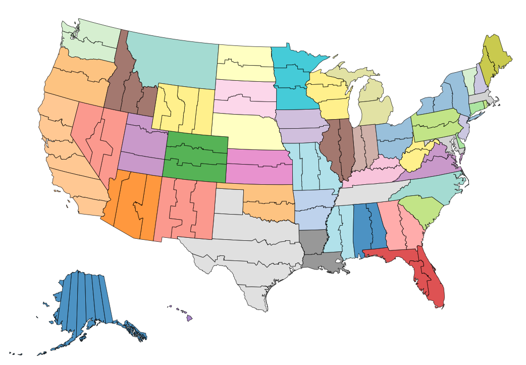
The State Plane Coordinate System (SPCS) is the most widely used plane coordinate system for surveying, engineering, and cadastral work in the United States. SPCS divides the country into zones, each with its own set of parameters for mapping, ensuring high accuracy for local-scale applications. SPCS splits the country into 120 zones, each tailored to a single state or portion of a state (Figure 4). To maintain low distortion within each zone, a Cartesian grid is superimposed with an origin shifted far enough west and south to keep all coordinate values positive. While the projection framework is consistent nationwide, the measurement units differ by state —some use U.S. survey feet, others use meters, and several support both to maintain compatibility between legacy and modern datasets. For example, California, Texas, and New York traditionally publish SPCS coordinates in U.S. survey feet, while Illinois and Minnesota use meters exclusively. Florida allows both feet and meter versions, depending on agency preference. This variation reflects each state’s historical surveying practices and transition pace toward metric standards. Each zone maintains linear distortion below 1 part in 10,000, making SPCS ideal for surveying, engineering, and cadastral applications in a local scale.

SPCS zones are based on two main map projections depending on the zone’s geographic orientation. A zone that extends primarily north-south uses the Transverse Mercator projection; one that stretches east-west uses a Lambert Conformal Conic projection. These projections are selected to align with the dominant axis of each zone to minimize distortion across the mapped area. In both cases the projection’s central meridian (or pair of standard parallels) is placed near the zone’s midpoint to balance scale error on either side.  This alignment ensures that the grid reflects true distances and directions with high accuracy, especially in regions like Colorado, which is divided into multiple Lambert-based zones to maintain consistency across its east-west extent.

Every zone then gains its own Cartesian grid. Surveyors establish a false origin some fixed distance, which is about 2 000 000 ft (or 500 000 m) west of the central meridian and south of the zone’s southern edge so that all coordinates inside the zone remain positive. Distances measured east of this origin are eastings (x), and those measured north are northings (y); units are feet in legacy datasets and meters in many NAD 83 implementations.

The U.S. Geological Survey 7.5-minute quadrangles printed between 1947-1995 show SPCS ticks and collar notes tied to NAD 27, which can differ from modern NAD 83/WGS 84 positions by several hundred meters. Later US Topo editions (2010-2016) carried NAD 83 State Plane ticks, but these were removed after 2017 as digital GIS supplanted paper grids. Modern GIS software and many field GPS/GNSS apps can still display SPCS coordinates for high-precision land surveying, engineering design, and other local-scale mapping tasks where sub-meter accuracy is important. In contrast to SPCS, the Universal Transverse Mercator (UTM) system applies a single projection method, the Transverse Mercator projection, in a consistent manner worldwide. The Earth is divided into 60 longitudinal zones, each 6 degrees wide, with a secant version of the projection applied to reduce distortion. A scale factor of 0.9996 is used at the central meridian to keep distortion below 1 part in 2,500 (0.04%) near the center of each zone. Like SPCS, UTM overlays a Cartesian grid on each projected zone, using false easting and northing values to ensure positive coordinates. This consistent global framework allows UTM to support a wide range of spatial data applications, particularly for regional mapping and GPS-based positioning.

As the National Geodetic Survey (NGS) introduced the third generation of the State Plane Coordinate System to reflect new datums and technological advancements. This modernization led to the development of the State Plane Coordinate System of 2022 (SPCS2022). It replaces the NAD 83 datum with coordinates referenced to the new North American Terrestrial Reference Frame of 2022 (NATRF2022). Unlike earlier versions, SPCS2022 allows states to define custom zones to better match their mapping and surveying needs by improving accuracy and flexibility. Some states have adopted multiple low-distortion projection zones, while others maintain a single statewide zone. SPCS2022 uses metric units by default, but state-specific implementations may also support U.S. survey feet for local consistency.

The introduction of SPCS2022 is part of a broader national modernization effort by NGS to redefine the geodetic reference framework of the United States. This effort replaces the long-standing North American Datum of 1983 (NAD 83) and the North American Vertical Datum of 1988 (NAVD 88) with new, fully GNSS-based reference frames. The new systems—the North American Terrestrial Reference Frame of 2022 (NATRF2022) and the North American–Pacific Geopotential Datum of 2022 (NAPGD2022)—use continuously operating GNSS reference stations instead of fixed survey monuments. This update corrects known biases, such as NAD 83’s approximate two-meter offset from the Earth’s center of mass and integrates precise geoid modeling to define both horizontal and vertical positions more accurately. Together, these new datums will underpin all modern spatial reference systems, including SPCS2022. 

3.3 Accuracy and Distortion in Plane Coordinates

The Universal Transverse Mercator (UTM) system is based on a secant Transverse Mercator projection with a scale factor of 0.9996 at the central meridian. This design keeps linear distortion below 1 part in 2,500 (0.04%) within approximately ±3° of the central meridian, though distortion increases toward the edges of each 6° zone—typically remaining under 1 part in 1,000 up to ±4.5°. Due to its larger zone size, UTM introduces slightly greater linear distortion compared to the State Plane Coordinate System (SPCS), particularly in areas near zone boundaries. Like SPC, UTM is also subject to ground-to-grid discrepancies when elevations deviate from the projection surface. Despite these limitations, UTM remains highly effective for regional mapping due to its global consistency and compatibility with GPS and GIS platforms.

3.4 USGS's Choice of UTM for the National Map

The U.S. Geological Survey selected the UTM system as the standard for its National Map because it provides a consistent, metric-based reference framework across the entire country. UTM coordinates are globally recognized and widely supported by GPS and GNSS devices, and the system aligns well with the WGS 84 datum used in modern remote sensing and imagery platforms. Despite these advantages, UTM also presents some challenges. Zone boundaries can divide large-area datasets, and scale variation across a zone can complicate certain analyses. Additionally, users who are familiar with localized systems, such as the State Plane Coordinate System (SPCS), may find UTM less intuitive. Alternatives such as SPC or a single national Lambert projection reduce cross-zone issues and offer more localized precision but lack the international compatibility and straightforward metric framework that made UTM the preferred choice for a national-scale base map.

In recognition of these limitations, specialized referencing systems have been developed to fulfil specific operational needs. The Military Grid Reference System (MGRS), for instance, builds on the Universal Transverse Mercator (UTM) by translating numerical coordinates into concise alphanumeric strings, thus facilitating quick and precise communication in military or emergency situations. Locations in MGRS are identified by a combination of Grid Zone Designators, designations for 100,000-meter squares, and numerical eastings and northings, with their length varied in relation to the desired precision. Similarly, the World Geographic Reference System (GEOREF) was developed for primary application in aviation on a latitude-longitude grid with alphanumeric coordinates. GEOREF, in contrast to UTM and MGRS, has worldwide coverage under one system but lacks UTM's metric precision and rigorous control of distortion. Thus, every referencing system prioritizes various operational needs: UTM is concerned with spatial accuracy and appropriateness to detailed GIS analysis, MGRS with quick, unambiguous communitcation within operational environments, and GEOREF with large-area navigation and worldwide simplicity of use.

4. National Grid Systems and The U. S. National Grid

Many countries have developed national grid systems tailored to their geodetic datums and mapping needs. These systems often simplify UTM or other projected coordinates into formats that are easier to use in practice, especially for local navigation and mapping. For example, the British National Grid, also known as The Ordnance Survey National Grid reference system (OSGB), uses an alphanumeric Transverse Mercator system based on the OSGB36 datum, while Ireland’s ITM grid and Australia’s Map Grid of Australia (MGA) adapt the UTM framework with simplified numeric coordinates. Despite differences in projection and precision, these systems share key features: a consistent national datum, truncation rules, and formats that prioritize usability over raw coordinate values.

While UTM provides a consistent spatial reference, its numerical format typically consists of long strings of numbers, which can be complicated and confusing for non-specialists. To address this challenge, the U.S. National Grid (USNG) was developed as a simplified version of UTM, making location referencing more accessible for practical applications such as emergency response, land navigation, and public safety. According to the Federal Geographic Data Committee (FGDC), which oversees standards for USNG, this system simplifies UTM coordinates into a more user-friendly format. The FGDC’s official USNG website— United States National Grid — Federal Geographic Data Committee—offers helpful figures illustrating the structure and use of the USNG, showing how it improves readability and efficiency without sacrificing accuracy.

USNG is directly based on the Military Grid Reference Systems and has the same fundamental structure, based on WGS 84 datum and transverse Mercator projection, as UTM.

USNG retains the same underlying structure of using the WGS 84 datum and transverse Mercator projection but introduces a hierarchical format for expressing coordinates more intuitively. Each USNG location consists of three components:

1. Grid Zone Designation (e.g., 16T),
2. 100,000-meter square identifier (e.g., MJ),
3. Numerical easting and northing values, which can be truncated or extended for varying levels of spatial precision.

This structure allows users to communicate spatial locations at varying levels of detail, from general regions to precise points within a few meters, without overwhelming numbers.

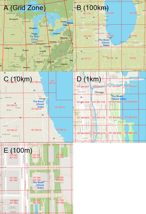
For example, consider Cloud Gate in Chicago, Illinois:

• Grid Zone Designation (GZD): 16T (Figure 5.A)
• 100,000-meter square: 16T DM (Figure 5.B)
• 10,000-meter square: 16T DM 43 (Figure 5.C)
• 1,000-meter square: 16T DM 4836 (Figure 5.D)
• 100-meter square: 16T DM 482 369 (Figure 5.E)

In this example, “16T” is the Grid Zone Designation, identifying UTM Zone 16 North and the latitude band “T.” The latitude band letters (from C at 80°S to X at 84°N) indicate north–south position within the UTM framework and help distinguish areas with the same zone number in different hemispheres. “DM” is the 100 000-meter square identifier, designating a specific grid square within Zone 16T. Together, “16T DM” defines a unique 100 × 100 km region on the ground, within which the numeric easting (482) and northing (369) values locate a more precise position.

With this kind of nested precision, responders and map users can communicate the location of interest with as much or as little detail as needed. For emergency management, search-and-rescue, or disaster relief teams, USNG dramatically improves coordination by using intuitive and shorter location references, minimizing errors in high-pressure situations. Moreover, USNG is fully integrated into many GIS and GPS platforms, allowing users to switch between UTM and USNG formats seamlessly depending on operational needs.

Figure 5 illustrates how the U.S. National Grid refines spatial precision by subdividing each larger square into progressively smaller ones: (A) 100 km, (B) 10 km, (C) 1 km, and (D) 100 m. Each level nests within the one above it, showing how the coordinate notation shortens or expands to match the needed precision for mapping or field operations.

References

- Battersby, S. (2017). Map Projections. The Geographic Information Science & Technology Body of Knowledge (2nd Quarter 2017 Edition), John P. Wilson (ed.)
- Bolstad, P., and Manson S. (2022). GIS Fundamentals: A first text on geographic information systems (Seventh edition). Elder Press.
- Burrough, P. A. and McDonnell, R. (1998). Principles of Geographical Information Systems, 2nd Edition. Oxford: Oxford University Press.
- Chang, K.-T. (2019). Introduction to Geographic Information Systems, 9th Edition. McGraw-Hill Education, New York, NY.
- Chrisman, N. R. (2002). Exploring Geographic Information Systems, 2nd edition. New York, NY: Wiley.
- Clarke, K. C. (1999). Getting Started with Geographic Information Systems (2nd edition). Upper Saddle River, New Jersey, USA: Prentice Hall.
- DeMers, M.N. (2008). Fundamentals of Geographical Information Systems (4th Edition). John Wiley & Sons.
- Faculty ITC, the University of Twente. (2020). Projected coordinate systems. The Core of GIScience 2020. ITC Learning Teaching Base, University of Twente.
- Federal Emergency Management Agency (FEMA). (2011). U.S. National Grid (USNG) Implementation Guide. U.S. Department of Homeland Security.
- Fukushima, T. (2006). Transformation from Cartesian to geodetic coordinates accelerated by Halley’s method. Journal of Geodesy 79:689–693.
- Haklay, M. (2010). Interacting with Geospatial Technologies. UK: John Wiley & Sons.
- Hearnshaw, H. M., & Unwin, D. J. (Eds.). (1994). Visualization in Geographic Information Systems. Wiley.
- Johnson, L. L., Pettersson, C. B., & Fulton, R. E. (Eds.). (1999). GIS and mapping practices and standards: Proceedings of a symposium (ASTM STP 1345). ASTM International.
- Laurini, R., & Thompson, D. (1992). Fundamentals of Spatial Information Systems. Academic Press.
- Maune, D. F. (Ed.). (2007). Digital elevation model technologies and applications: The DEM users manual (2nd ed.). American Society for Photogrammetry and Remote Sensing (ASPRS).
- Obermeyer, N. J., & Pinto, J. K. (1994). Managing Geographic Information Systems, 1st Edition. New York, NY: Guilford Press.
- Onsrud, H. J., & Cook, G. (Eds.). (1991). Geographic and Land Information Systems for Practitioners. American Society for Photogrammetry and Remote Sensing (ASPRS).
- Seong, J. C. (2023). Coordinate Transformations. The Geographic Information Science & Technology Body of Knowledge (4th Quarter 2022 Edition), John P. Wilson (ed.)
- Theobald, D. M. (2003). GIS Concepts and ArcGIS Methods. Conservation Planning Technologies, Inc.
- United States National Grid (USNG) Center. (n.d.). US National Grid (USNG).
- Wikipedia contributors. (2024, June 13). Projected coordinate system. Wikipedia.
- Wisconsin Land Information Association. (2021, May 14). Introduction to U S National Grid [Video]. (Speaker: Randy Kippel). YouTube.
Learning outcomes
-
33 - Associate SPC coordinates and zone specifications with corresponding positions on a U.S. map or globe
34 - Associate UTM coordinates and zone specifications with corresponding position on a world map or globe
221 - Discuss the pros and cons of the U.S. Geological Survey's choice of UTM as the standard coordinate system for the U.S. National Map
519 - Describe the characteristics of the "national grids" of countries other than the U.S.
767 - Differentiate the characteristics and uses of the UTM coordinate system from the Military Grid Reference System (MGRS) and the World Geographic Reference System (GEOREF)
854 - Discuss the magnitude and cause of error associated with SPC coordinates
855 - Discuss the magnitude and cause of error associated with UTM coordinates
1226 - Explain what State Plane Coordinates system (SPC) eastings and northings represent
1229 - Explain what Universal Transverse Mercator (UTM) eastings and northings represent
1244 - Explain why plane coordinates are sometimes preferable to geographic coordinates
1362 - Identify the map projection(s) upon which SPC coordinate systems are based, and explain the relationship between the projection(s) and the coordinate system grids
1363 - Identify the map projection(s) upon which UTM coordinate systems are based, and explain the relationship between the projection(s) and the coordinate system grid
1543 - Recommend the most appropriate plane coordinate system for applications at different spatial extents and justify the recommendation
1971 - Describe how Cartesian grids are used in planar coordinate systems to assign unique locations based on x (eastings) and y (northings) coordinates.
1976 - Summarize the benefits of the U.S. National Grid (USNG) in emergency response and field operations.