[DM-03-075] Defining and Designing Spatial Queries
Spatial information retrieval is fundamental in modern applications that enhance data analysis by enabling the representation, storage, and management of spatial data. Spatial database systems and Geographical Information Systems are essential tools for those applications, offering efficient spatial data representation and spatial query processing. Spatial data is usually represented by geometries in Euclidean space, such as points, lines, and regions. Spatial query processing mainly relies on the task of retrieving spatial objects meeting specific spatial conditions. These conditions are often defined by spatial relationships, which describe how spatial objects relate within a given space and have different semantics, such as topological relationships (e.g., overlap, inside), metric relationships (e.g., distance), and direction relationships (e.g., cardinal directions). A typical spatial query finds all objects in a specified relationship with a search object. This article systematically explores the design and definition of spatial queries by using spatial relationships as their main foundation. By introducing both intuitive and formal definitions of various types of spatial queries, it helps users to understand each query’s practical use and underlying mechanics.
Tags
Author & citation
Carniel, A. C. (2025). Designing and Defining Spatial Queries. The Geographic Information Science & Technology Body of Knowledge (2025 Edition), John P. Wilson (ed). DOI: 10.22224/gistbok/2025.1.12.
Explanation
- Introduction
- Classes of Spatial Queries
- Topology-based Spatial Queries
- Metric-based Spatial Queries
- Direction-based Spatial Queries
- Spatial Join Queries
- Conclusions
Spatial information retrieval is a pivotal component in modern, cutting-edge applications that enhance data analysis by integrating the representation, storage, and management of spatial or geometric data. For instance, spatial data science applications, such as environmental monitoring, urban planning, and epidemiological studies, often require extracting insights from complex spatial datasets by retrieving spatial information that meets specific constraints. Similarly, spatial crowdsourcing applications, such as ride-sharing and on-demand services, rely on efficiently processing spatial queries for different use cases, such as real-time routing and demand balancing. In disaster management, spatial information retrieval is essential for extracting real-time spatial data from remote sensing technologies, enhancing applications such as flood prediction, wildfire monitoring, and emergency response. Additionally, location-based services employ spatial queries for personalized recommendations, navigation, and urban mobility solutions, improving user experiences. In essence, spatial information retrieval serves as a foundational element of Geographic Information Science and Technologies, enabling efficient access, processing, and utilization of spatial data across diverse domains and applications.
In essence, spatial information retrieval serves as a foundational element of Geographic Information Science and Technologies, enabling efficient access, processing, and utilization of spatial data across diverse domains and applications.
Spatial database systems and Geographical Information Systems (GIS) play an essential role in enabling efficient spatial information retrieval by offering two key features: (i) spatial data representation, and (ii) spatial queries. As for the spatial data representation, these systems store and handle spatial or geographic information represented by geometries in the Euclidean space in the form of spatial objects. Such objects are instances of vector-based data types known as spatial data types, which include two-dimensional points, lines, and regions (also called polygons). Spatial objects can assume simple or complex structures. Simple spatial objects are single-component objects, whereas complex spatial objects contain finitely many components that allow users to represent the reality and complexity of geographic phenomena. Examples of spatial objects include landmarks such as monuments and historical sites represented as point objects, utility networks like water pipes and electrical lines denoted as line objects, and geographical features like lakes and forests shaped as region objects. Figure 1 depicts a small spatial dataset containing 11 simple point objects (p1 to p11), four simple line objects (l1 to l4), and seven simple region objects (r1 to r7).
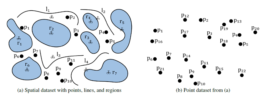
With respect to spatial queries, spatial database systems and GIS are responsible for processing user queries (e.g., through SQL) that retrieve spatial objects satisfying a particular set of spatial conditions. Such conditions are typically expressed by spatial relationships, which outline how two or more spatial objects relate to each other within a given space. In this sense, spatial relationships provide the fundamental semantics of spatial queries, allowing users to formulate queries that return all spatial objects in a given relationship with a search object (also known as reference object or query object), which is another spatial object provided by the user or supplied as input by the application. The spatial dataset shown in Figure 1a is employed in this article to illustrate how several types of spatial queries work. Since some types of spatial queries focus on handling point objects, the center of mass of line and region objects from Figure 1a (shown as dashed points) together with the point objects define the point dataset shown in Figure 1b, which is used to illustrate such types of spatial queries.
This article pursues the goal of explaining a systematic approach of designing and defining spatial queries by using spatial relationships as their main foundation. In the literature, it is possible to identify three main types of spatial relationships (Worboys, 1992, Güting, 1994, Tinghua and Yaolin, 2003, Carniel, 2024), each providing a unique perspective on how spatial objects interact; they are: (i) topological relationships, (ii) metric relationships, and (iii) direction relationships. In this article, they are employed to design spatial queries, leading to the following corresponding classes of spatial queries: (i) topology-based spatial queries, (ii) metric-based spatial queries, and (iii) direction-based spatial queries. Moreover, when manipulating two sets of spatial data, spatial join queries are designed, which match spatial objects from two spatial datasets based on the semantics of spatial relationships. In essence, this article focuses on designing spatial queries that retrieve vector-based, two-dimensional spatial objects (as shown in Figure 1), using spatial relationships as the primary filters. Without loss of generality, the query examples provided in this article mainly manipulate simple spatial objects for the sake of simplicity. The formal definitions presented in this article are generic and can be applied to spatial datasets containing complex spatial objects, as long as the underlying spatial relationship supports them. Other types of spatial queries and the manipulation of different spatial data models are beyond the scope of this article and are briefly outlined in Section 7.
The rest of this article is organized as follows. Section 2 presents a systematic classification of spatial queries (or taxonomy) and summarizes the notations employed in this article to formally define the spatial queries. Subsequently, each spatial query class (Sections 3 to 5) is introduced by consecutively providing (i) basic concepts from its underlying type of spatial relationship, (ii) intuitive descriptions of the underlying semantics of the spatial query class, and (iii) formal definitions of types of spatial queries belonging to the class. Section 6 presents intuitive descriptions and formal definitions of spatial join queries. It is important to note that the goal is not to provide an exhaustive and comprehensive description of all types of spatial queries but discuss common spatial queries employed in applications. More definitions and discussions in this field can be found in (Carniel, 2024). Finally, Section 7 concludes the article and sketches research directions in the area.
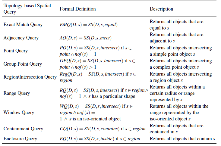
Table 1 presents the taxonomy that classifies spatial queries (Carniel, 2024). Each class comprises a set of query templates (i.e., types of spatial queries) based on the usage of spatial relationships. This means that each class in the left column of Table 1 is a superclass that categorizes types of spatial queries frequently found in applications. These types of spatial queries are formally defined in the following subsections by using the notations shown in Table 2.
Table 1. Classification of spatial queries. The classes are based on the types of spatial relationships in the design and definition of the queries (Carniel, 2024).
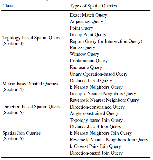
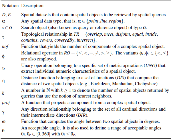
Table 2. Notations and symbols employed in this article to formally define the classes of spatial queries.
3. Topology-based Spatial Queries
3.1 Underlying Concepts
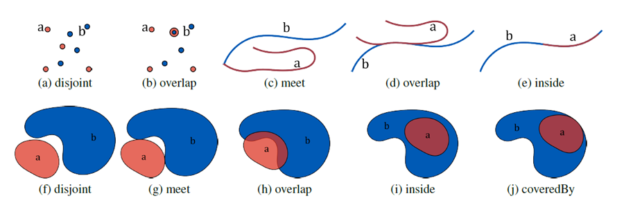
The design of topology-based spatial queries relies on the usage of topological relationships. A topological relationship characterizes the relative position of two spatial objects and are invariant under topological transformations like translation, scaling, and rotation. The 9-intersection model (9-IM) (Egenhofer and Herring, 1990; Schneider and Behr, 2006; Shen et al., 2018) is a well-accepted concept that uses point sets and point set topology to define a complete collection of mutually exclusive topological relationships for each combination of simple and complex spatial data types. This model creates a matrix to represent the nine possible intersections of the boundary, interior, and exterior of two spatial objects, according to the topologically invariant criteria of emptiness and non-emptiness. This model can be extended to leverage the dimensions of the intersections (Clementini and Felice, 1995; McKenney et al., 2005) to refine the expressiveness of the topological relationships. Due to the large number of relationships that can be obtained by the 9-IM (i.e., each valid matrix is a topological relationship), similar relationships are commonly merged into a single relationship (Schneider and Behr, 2006). As a result, the following eight topological relationships are defined: overlap, meet, disjoint, equal, inside, contains, covers, and coveredBy. The Open Geospatial Consortium includes a ninth relationship named intersect to express that two objects are not disjoint. In essence, these topological relationships are implemented as Boolean spatial operators in spatial database systems and GIS.
Figure 2 depicts some examples of topological relationships between points, lines, and regions. Note that other examples can be directly derived from this figure. For instance, the topological relationship intersect requires that at least one point be shared between two objects (i.e., they should not be disjoint); this means that Figures 2b-e and 2g-j show examples of this predicate as well. For the relationships contains and covers, they are the converse of the relationships inside and coveredBy, respectively. This means that inside(a,b) = contains(b,a) and coveredBy(a,b) = covers(b,a) for two spatial objects a,b. Illustrative examples of topological relationships for all type combinations can be found in Schneider and Behr (2006).
3.2 Intuitive Description
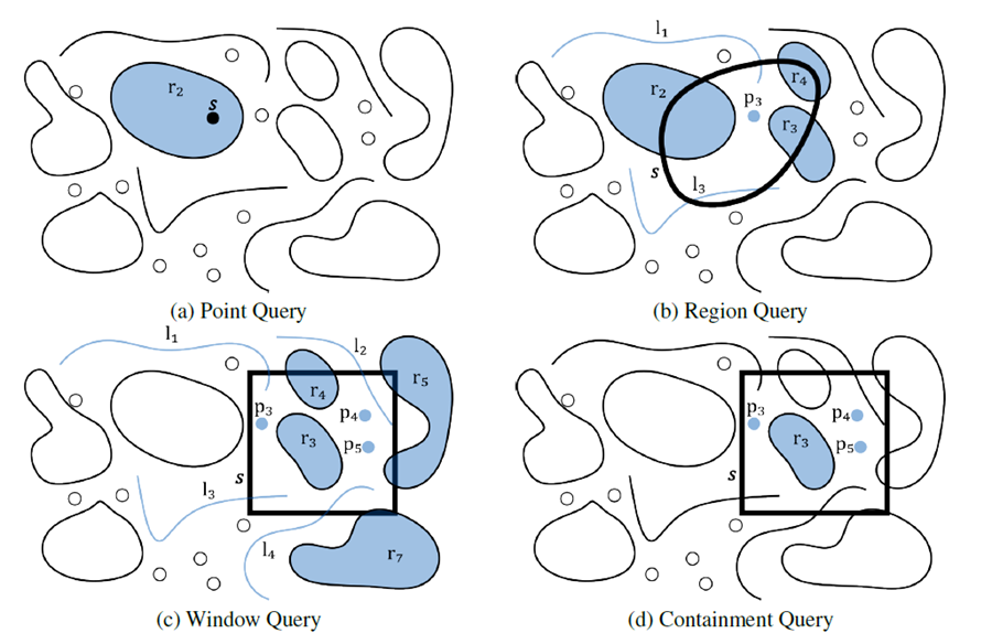
A topology-based spatial query can be expressed by the following spatial selection: “find all spatial objects from a spatial dataset D in a given topological relationship with the search object s” (Gaede and Günther, 1998; Carniel et al., 2020). Specific types of spatial queries are identified by specifying a particular topological relationship for
and restricting the spatial data type of s. By using the running example (Figure 1a), Figure 3 depicts some examples of topology-based spatial queries.
3.3 Formal Definitions
Let be a topological relationship in TR = {overlap, meet, disjoint, equal, inside, covers, coveredBy, intersect}. Each topological relationship has the signature
. The formal definition of a spatial selection is given in Equation 1 as follows:
The spatial selection SS is used to design types of topology-based spatial queries by assuming particular values and properties for and s, as depicted in Table 3. The The topology-based spatial queries shown in this table take D and s as inputs and invoke SS with a specific value for and possible constraints to s if needed. Further, it is possible to establish the direct association of the meaning of the topological relationship to the semantic of the spatial query. Each query example in Figure 3 shows th search object s and highlights the resultling spatial objects as follows: (i) the Point Query returns r2, (ii) the Region Query retrieves p3, l1, l3, and r2 to r4, (iii) the Window Query returns p3 to p5, l1 to l4, r3 to r5, and r7, and (iv) the Containment Query yields p3 to p5 and r3.
Table 3. Types of topology-based spatial queries defined by using the underlying spatial selection from Carniel (2024): .
4. Metric-based Spatial Queries
4.1 Underlying Concepts
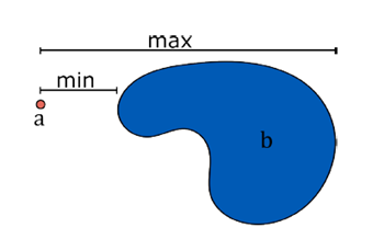
The design of metric-based spatial queries makes use of metric relationships. A metric relationship indicates how two spatial objects are related by using numerical measures (Güting, 1994). These measures can be viewed from two perspectives. The first involves the intrinsic numerical properties of spatial objects, such as the area and perimeter of a region object and the length of a line object. The second perspective relates to the proximity between two spatial objects based on some distance function. Commonly, the minimum distance and the maximum distance (i.e., length of the longest line between points of two spatial objects) are deployed when designing spatial queries. Figure 4 contrasts the minimum and maximum distances between a point object and region object.
4.2 Intuitive Descriptions
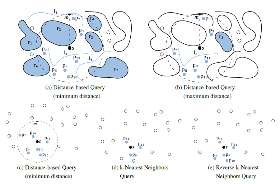
Metric-based spatial queries can be divided into the following three groups: (i) spatial queries with unary operators, (ii) spatial queries with binary operators, and (iii) the retrieval of nearest neighbors. The first group includes queries that relate two or more spatial objects by comparing their individual intrinsic numerical properties given by unary operators, such as the area of region objects and the length of line objects. The second group encompasses distance-based spatial queries, which deploy binary operators to compute the distance between two spatial objects. Finally, the last group encompasses queries that retrieve a number of objectsthat are the nearest neighbors of a particular spatial object (Taniar and Rahayu, 2013). Figure 5 depicts some practical examples of metric-based spatial queries by using both datasets of the running example.
4.3 Formal Definitions
Let be a relational operator in RO =
. Let UNO be the set of possible unary operators that extract an individual numeric property of a spatial object such that each operator has the signature α→R. The first group of metric-based spatial queries is generalized by the Unary Operation-based Query, which retrieves all spatial objects from D that have a numerical property satisfying a given relational expression with the same type of numerical property of the search object s. It can be formally defined by Equation 2 below:
Equation 2:
In both cases, can be a type-dependent unary operator, which requires a specific spatial data type for its operand. For instance, if
{area, perimeter}, it indicates that the operand has to be a region object. Similarly for
{length}, its operand must be a line object. To adequately handle this situation, an additional condition should be included in the definition of UOQ (Equation 2) to guarantee valid results. This condition evaluates the correspondence between the accepted data types by
and the data type of the spatial objects of D and s.
The second group of metric-based spatial queries is generalized by the Distance-based Query, which returns all spatial objects from D at a certain distance from the search object s. Let DIS be the set of possible functions that compute the distance of two spatial objects (e.g., minimum distance, maximum distance) such that each function has the signature
. Let
. The Distance-based Query is formally defined by Equation 3:
Figures 5a-c show examples of Distance-based Queries, where the parameter m denotes the distance from the search object s. The distance function plays an important role when interpreting a Distance-based Query, especially when dealing with line and region objects. For instance, Figures 5a-b have the same search object s but apply different distance functions. While the query in Figure 5a uses the minimum distance and returns almost all objects (except p1, p4 to p6, l2, and r5), the query in Figure 5b employs the maximum distance and retrieves nine objects (i.e., p2, p3, p7 to p11, l3, and r3) that are completely within the distance specified by m. This is the case since the maximum distance function is based on the longest line between the points of two spatial objects. Figure 5c shows another example of Distance-based Query by considering the point dataset of the running example (Figure 1b), returning the points p7 to p11 and p14.
In addition, the previous function DQ (Equation 3) can have different variants leading to different semantics. By replacing the relational operator with
, a stricter comparison is obtained since the boundary of the range will not be considered in the evaluation. Further, the use of the operator
(and similarly
) leads to the retrieval of those objects that are not at a certain distance from the search object s.
The third group of metric-based spatial queries focuses on returning the nearest neighbors to a given spatial object. Let with
. The k-Nearest Neighbors Query finds a set of spatial objects from D that are the K-nearest neighbors of the search object s. This query can be formally expressed by Equation 4:
Equation 4: 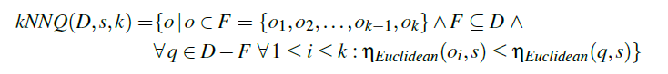
Figure 5d depicts one example of k-Nearest Neighbors Query applied to the point dataset of the running example that returns the three nearest points to the search object s (i.e., p9, p11, and p14). This query has some variants, such as the Group k-Nearest Neighbors Query which allows the search object to be a complex object with several components (i.e., nof (s) > 1). Commonly, this is a complex point object. The goal of this query is to retrieve the k spatial objects from D with the smallest sum of distances to every component of s. Let proj be a function that gets a specific component from a complex spatial object. For instance, proj(s,1) yields the first component of the object s. The Group k-Nearest Neighbors Query is formally defined by Equation 5 as follows:
Equation 5: 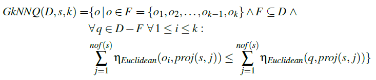
Another variant is the Reverse k-Nearest Neighbors Query, which retrieves all spatial objects from D that have the search object s as one of their k-nearest neighbors. It can be formally written by the Equation 6 as follows:
5. Direction-based Spatial Queries
5.1 Underlying Concepts
The design of direction-based spatial queries employs direction relationships. A direction relationship describes how two spatial objects are related by examining directional measures, such as angular ranges and cardinal directions (e.g., north and south). These relationships intuitively help determine whether a spatial object is positioned in a particular direction with respect to another spatial object. Various methods can be employed to derive direction relationships between two spatial objects. One notable conceptual method to derive direction relationships is the direction-relation matrix (Goyal and Egenhofer, 1997), which divides the space surrounding a reference object (e.g., the search object) into nine regions (eight cardinal directions and a central region) and captures the possible interactions between these regions and another spatialobject. This matrix can be augmented by segmenting the space around both operand objects and merging the resulting regions into an objects interaction matrix (Schneider et al., 2012). In addition to cardinal directions, applications may also focus on processing direction relationships based on user-defined angles and angular ranges, such as the visible area of a spatial object. Figure 6 illustrates examples of direction relationships using cardinal relations.
5.2 Intuitive Descriptions
The general purpose of direction-based spatial queries is to find all spatial objects in a given particular direction from the search object. It is possible to identify two main types of spatial queries belonging to this class: (i) spatial queries based on (inter)cardinal directions (e.g., north, south, west, east, and their intermediate directions), and (ii) spatial queries retrieving spatial objects in a particular angular range. The first type considers that the direction is fixed and commonly expressed by the four cardinal directions and their intermediate directions.
The second type generalizes the first one by accepting any particular angular range (also known as the visible angle). Figure 7 depicts some practical examples of direction-based spatial queries by using the point dataset of the running example (Figure 1b).
5.3 Formal Definitions
Let DIR be the set of functions that compute the cardinal directions (i.e., north, east, south, west) and intercardinal directions (i.e., northeast, southeast, southwest, and northwest), as well as their intermediate directions (e.g., west-northwest, north-northwest) of two spatial objects such that DIR has the signature
. The first type of spatial query of this class is called Direction-constrained Query, which retrieves all spatial objects in a given direction of s. This query can be formally described by Equation 7 as follows:
Equation 7:
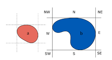
In essence, this query has a strict evaluation of the direction of two spatial objects by using the operator . This is due to the representation of the (inter)cardinal directions as specific angles. For instance, the azimuth angle equal to 0◦ denotes that one object is to the north of another object. Figure 7a shows one example of Direction-constrained Query by considering a iso-oriented search object s where the operator γ corresponds to the evaluation of the cardinal direction east, retrieving the points p3 to p5, p17, p18, and p20.
The second type of direction-based spatial queries generalizes the Direction-constrained Query to get a particular angle as input instead of using . This generalization leads to the Angle-constrained Query, which finds all spatial objects that have a particular angular relationship with s. Let
be a function that computes the angle between two spatial objects and has the signature
. Let further
to denote a particular angle in degrees (or
. The Angle-constrained Query can be defined by Equation 8 as follows:
In Equation 8, the angular relationship checks whether the angle between two spatial objects satisfies an equality condition with an input value. However, this equality check is very strict. Let to specify the range of acceptable angles (also known as angular range). By employing
, it is possible to determine whether the left and right side of the angular range is open (<) or closed (≤). Hence, Equation 8 can be generalized as the following Equation 9:
It is important to note that the last four parameters allow users to define closed intervals (i.e., ), left open intervals (i.e.,
), right open intervals (i.e.,
and open intervals (i.e.,
). Figure 7b shows one example of this type of query, returning the points p9 to p11, p14, and p15. The query in this figure uses open intervals
where
represent angles measured clockwise from the North of the search object (i.e., these angles follow the azimuth angle convention relative to the search object s).
6.1 Intuitive Descriptions
The spatial join is a typical operation that associates multiple spatial datasets and has been widely studied in the literature (Gaede and Günther, 1998). Given two spatial datasets D and E, a spatial join query retrieves the pairs of spatial objects that satisfy a given spatial relationship or a combination of spatial relationships. This means that the spatial queries previously specified and discussed in Sections 3, 4, and 5 can be generalized to deal with two spatial datasets by considering that the search object s is now a set of spatial objects.
6.2 Formal Definitions
Table 4 introduces typical types of spatial joins frequently found in spatial applications and studied in the literature (Jacox and Samet, 2007: Li and Taniar, 2017; Carniel, 2024). A spatial join can be formally written by the following general template shown in Equation 10:
where [cond] is replaced by a set of conditions as depicted in the third column of Table 4. This means that the type of a spatial join query is distinguished by the employed spatial relationships. Specific parameters can be given by the user to execute a spatial join query. Recall that denote a topological relationship in TR, a distance function in DIS, and the computation of the angle between two spatial objects, respectively (Sections 3, 4, and 5).
Table 4. Some variants of spatial join queries where JQ stands for Join Query (Carniel, 2024). The definitions are based on the template where [cond] should be replaced by the specified conditions of the spatial query.
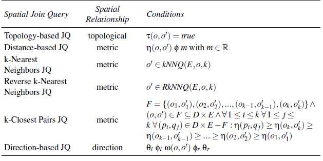
Intuitively, the Topology-based Join Query finds all pairs that satisfy a given topological relationship. For instance, all the intersecting pairs of D and E. The Distance-based Join Query retrieves all pairs that are spatially separated according to a given distance. The k-Nearest Neighbors Join Query retrieves the k closest neighbors of each spatial object of the first spatial dataset. This query is also known as All-Nearest-Neighbors Query. The Reverse k-Nearest Neighbors Join Query captures all objects from E together with their resulting objects from the execution of the Reverse k-Nearest Neighbors Query. In the same context of metric relationships, the k-Closest Pairs Join Query yields the k pairs with the minimum distances among all possible pairs. Finally, the Direction-based Join Query applies direction relationships to retrieve all pairs with the same angular range. Other types of spatial joins can also be designed by using different spatial relationships in their definitions.
This article has presented the intuitive description and formal definitions of various types of spatial queries, which can be classified according to how these queries incorporate spatial relationships into their core semantics and definitions. The following classes are identified: (i) topology-based spatial queries (based on topological relationships), (ii) metric-based spatial queries (based on metric relationships), and (iii) direction-based spatial queries (based on direction relationships). They have the common goal of retrieving spatial objects from a spatial dataset that satisfy specific constraints with respect to a search object. An additional class named spatial join queries is identified when the search object is generalized to a spatial dataset.
Spatial queries can also blend two or more types of spatial relationships, leading to queries with refined filter semantics. The three types of spatial relationships discussed in this article can be combined by using logical operators (i.e., or, and, not) to define new spatial queries. For instance, a spatial query that combines a Direction-based Spatial Query and Metric-based Spatial Query to “find all objects located in a particular direction (or acceptable angles) and limited to a given distance in relation to the search object.” In addition, there are several approaches in the literature that augment the meaning and interpretation of topological relationships by including metric and directional measurements in underlying models like the 9-intersection model. For instance, a spatial query that combines topology and metric notions can “find all line objects that run along the search object.” Another example is a spatial query that mixes topology and direction notions to “retrieve all line objects that run along the east boundary of the search object.” Moreover, other types of spatial queries can combine notions of distance and direction in their underlying definitions to create a query that “retrieves all nearest objects around the search object from different directions.” All these queries that combine two or more types of spatial relationships in their semantics can be grouped as Hybrid Spatial Queries, which are discussed in Carniel (2024).
From the implementation point of view, spatial database systems and GIS deploy spatial indexstructures to efficiently process spatial queries by excluding objects that cannot be part of the final result. Index structures like the R-tree and its variants (see surveys in Gaede and Günther (1998) and Carniel and Aguiar (2023) organize nearby spatial objects into groups, using approximations such as minimum bounding rectangles (MBR) to simplify the complex shape that spatial object may have. While these approximations speed up query processing (since the computation of spatial relationships on them is commonly cheap), they may introduce areas that do not belong to the original spatial object and thus, potentially causing inaccuracies in the spatial query processing. To address this, spatial queries are often processed in two steps (Gaede and Günther, 1998: Carniel et al., 2020: Carniel and Aguiar, 2023): a filter step that narrows down candidates using spatial indexes and a refinement step that effectively verifies the spatial relationships to produce accurate results. More discussions on spatial query processing models are given in Carniel (2024) and Gaede and Günther (1998).
Spatial information retrieval is a broad area. This article has dealt with the identification of spatial queries on static and crisp spatial objects since their locations do not change over time and their positions, boundaries, and interiors are well-known and precisely defined in space. On the other hand, spatial phenomena can be also represented by different models, such as spatial networks (Papadias et al., 2003), spatiotemporal data (Güting and Schneider, 2005; Schneider, 2017), fuzzy spatial data (Carniel and Schneider, 2021; Carniel et al., 2023), and high-dimensional data (Bohm et al., 2001, Teng et al., 2022). Spatial networks model systems like transportation, where queries might focus on connectivity or shortest paths. Spatiotemporal data captures changes over time, enabling queries that track or predict the movement of objects. Fuzzy spatial data captures the imprecise or uncertain nature of spatial information, requiring queries that handle vague boundaries and blurred interiors. Finally, high-dimensional data involves datasets with three dimensions or more, where queries must address the complexity of searching through those different dimensions. Therefore, each of these models introduces unique challenges for designing spatial queries, requiring specific spatial relationships tailored to their characteristics.
References
- Böhm, C., Berchtold, S., and Keim, D. A. (2001). Searching in highdimensional spaces: Index structures for improving the performance of multimedia databases. ACM Computing Surveys, 33(3):322–373.
- Carniel, A. C. (2024). Defining and designing spatial queries: the role of spatial relationships. Geo-spatial Information Science, 27(6):1868–1892.
- Carniel, A. C. and Aguiar, C. D. (2023). Spatial index structures for modern storage devices: A survey. IEEE Transactions on Knowledge and Data Engineering, 35(9):9578–9597.
- Carniel, A. C. and Schneider, M. (2021). A Survey of Fuzzy Approaches in Spatial Data Science. In IEEE International Conference on Fuzzy Systems, pages 1–6.
- Carniel, A. C., Ciferri, R. R., and Ciferri, C. D. A. (2020). FESTIval: A versatile framework for conducting experimental evaluations of spatial indices. MethodsX, 7:100695.
- Carniel, A. C., de Venancio, P. V. A. B., and Schneider, M. (2023). fsr: An r package for fuzzy spatial data handling. Transactions in GIS, 27(3):900–927.
- Clementini, E. and Di Felice, P. (1995). A comparison of methods for representing topological relationships. Information Sciences - Applications, 3(3):149–178.
- Egenhofer, M. J. and Herring, J. R. (1990). Categorizing binary topological relations between regions, lines and points in geographic databases. In The 9- Intersection: Formalism and Its Use for Natural-Language Spatial Predicates. National Center for Geographic Information and Analysis, University of California, Santa Barbara, CA.
- Gaede, V. and Günther, O. (1998). Multidimensional access methods. ACM Computing Surveys, 30(2):170–231.
- Goyal, R. K. and Egenhofer, M. J. (1997). The direction-relation matrix: A representation for directions relations between extended spatial objects. In The Annual Assembly and the Summer Retreat of University Consortium for Geographic Information Systems Science.
- Güting, R. H. (1994). An introduction to spatial database systems. The VLDB Journal, 3(4), 357-399.
- Güting, R. H. and Schneider, M. (2005). Moving objects databases. Morgan Kaufmann.
- Jacox, E. H., & Samet, H. (2007). Spatial Join Techniques. ACM Transactions on Database Systems (TODS), 32(1), 7.
- Li, L. and Taniar, D. (2017). A taxonomy for distance-based spatial join queries. International Journal of Data Warehousing and Mining, 13(3):1–24.
- McKenney, M., Pauly, A., Praing, R., and Schneider, M. (2005). Dimension-refined topological predicates. In ACM Int. Workshop on Geographic Information Systems, pages 240–249.
- Metcalf, L. and Casey, W. (2016). Metrics, Similarity, and Sets. In Metcalf, L. and Casey, W., editors, Cybersecurity and Applied Mathematics, pages 3–22. Syngress, Boston.
- Papadias, D., Zhang, J., Mamoulis, N., and Tao, Y. (2003). Query processing in spatial network databases. In VLDB Conference, pages 802–813.
- Schneider, M. (2017). Spatial and spatiotemporal data types as a foundation for representing space-time data in GIS. In Faiz, S. and Mahmoudi, K., editors, Handbook of Research on Geographic Information Systems Applications and Advancements, pages 1–28. IGI Global.
- Schneider, M. and Behr, T. (2006). Topological relationships between complex spatial objects. ACM Transactions on Database Systems, 31(1):39–81.
- Schneider, M., Chen, T., Viswanathan, G., and Yuan, W. (2012). Cardinal directions between complex regions. ACM Transactions on Database Systems, 37(2).
- Shen, J., Chen, M., and Liu, X. (2018). Classification of topological relations between spatial objects in two-dimensional space within the dimensionally extended 9- intersection model. Transactions in GIS, 22(2):514–541.
- Taniar, D. and Rahayu, W. (2013). A taxonomy for nearest neighbour queries in spatial databases. Journal of Computer and System Sciences, 79(7):1017–1039.
- Teng, D., Baig, F., Vo, H., Liang, Y., Kong, J., and Wang, F. (2022). 3DPro: Querying complex three-dimensional data with progressive compression and refinement. In International Conference on Extending Database Technology, pages 104–117.
- Tinghua, A. and Yaolin, L. (2003). Spatial relation resolution and spatial relation abstraction. Geo-spatial Information Science, 6(4):10–16.
- Worboys, M. F. (1992). A generic model for planar geographical objects. International Journal of Geographical Information Systems, 6(5):353–372.
Learning outcomes
-
1809 - Define key terms and notations associated with the formal definition of spatial queries and how they employ concepts from spatial data types and spatial relationships.
Define key terms and notations associated with the formal definition of spatial queries and how they employ concepts from spatial data types and spatial relationships.
-
1810 - Classify different types of spatial queries based on their spatial relationships, using a systematic taxonomy.
Classify different types of spatial queries based on their spatial relationships, using a systematic taxonomy.
-
1811 - Explain how spatial relationships establish the semantics of spatial queries.
Explain how spatial relationships establish the semantics of spatial queries.
-
1812 - Analyze the role of spatial relationships in designing and structuring spatial queries that affect the retrieval of spatial data in GIS and spatial database systems.
Analyze the role of spatial relationships in designing and structuring spatial queries that affect the retrieval of spatial data in GIS and spatial database syst