[AM-02-098] Boundaries and Zone Membership

Ter-Ghazaryan, D. (2025). Boundaries and Zone Membership. The Geographic Information Science & Technology Body of Knowledge (Issue 2, 2025 Edition).  John P. Wilson (ed.). DOI: 10.22224/gistbok/2025.2.14.

1. Introduction
2. Boundaries
3. Virtual Boundaries
4. Zones
5. Zonal Analysis
6. Crisp vs. Fuzzy Membership
7. Conclusion

1. Introduction

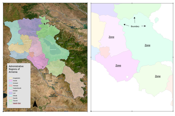
Boundaries and zones are fundamental concepts in GIS. They are used to represent spatial extents, divisions and relationships within geographic space. Boundaries demarcate the outlines of spatial units such as property parcels, political jurisdictions or ecological regions, whereas zones refer to the areas enclosed by those boundaries (Figure 1).

Across disciplines, the term “boundary” usually refers to a line or limit, while “zone” usually refers to an area or extent. Synonyms for both terms are many: border, edge, limit, contour for boundary; area, region, unit, sector for zone. Boundaries can be natural or human-made, physical/material or conceptual/virtual, and can be discrete, where there is a clear dividing line between zones, or fuzzy, where the transition is gradual. Zones are also subject to crisp and fuzzy membership. For crisp sets, membership is binary, i.e., an object either belongs to the set (membership=1) or it does not (membership=0), and for fuzzy sets membership is graded, i.e., an object can belong to a set partially, with a membership value anywhere between 0 and 1.

2. Boundaries

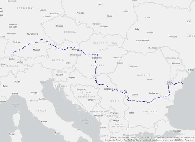
At its core, a boundary is a line that can be found between two distinct entities or zones. In geography, boundaries are lines or physical features that separate and delimit different geographic areas from each other and define the edges of various geographic regions or territories at various scales. Boundaries can be natural or human-made.  Natural boundaries are formed by recognizable physical features such as rivers, mountains or coastlines. Human-made boundaries include political and administrative boundaries which are defined by political processes, such as delimiting borders of countries or regions. Natural boundaries and human-made boundaries can sometimes coincide, as is the case with the Danube River forming a natural and political boundary between several countries in Europe—Hungary and Slovakia, Romania and Bulgaria, and others (Figure 2).

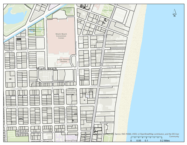
Boundaries can also separate administrative units and privately owned land parcels, and in the latter instance are called property boundaries or property lines. Property lines are an integral component of cadastral maps, and are essential for property taxation, land administration and management, real estate and urban planning (Figure 3).

In GIS, boundaries are typically represented as vector data, most often as lines or polylines. Lines or polylines are usually used to represent linear boundaries, such as roads, rivers or administrative or political borders. Representation and management of boundaries in GIS can be associated with some challenges, not all of which are technological. Among technological challenges are those of scale and generalization, as well as data quality and accuracy, whereas non-technological challenges include those related to ambiguity of borders and border disputes. In terms of scale and generalization, the level of detail in boundary representation depends on the map scale, especially on the scale at which the map was originally created. At smaller or coarser scales, boundaries become more generalized and less detailed, which can lead to loss of detail and accuracy. For example, the boundaries of a small island might be simplified at the scale of a world map, potentially leading to loss of accuracy and omission of certain features of the boundary.

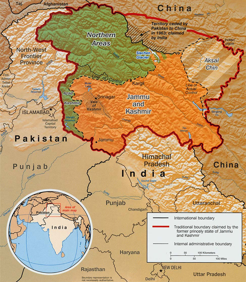
In terms of non-technological challenges, boundaries that form international borders between countries are not always clear-cut and accepted by all. Across the world, there are many instances of border disputes between neighboring countries, such as, for example, the Kashmir region, where both India and Pakistan claim overlapping territories, making the border a disputed boundary. In GIS, such disputed boundaries are typically represented with a dashed or dotted line to indicate the uncertainty or the contested nature of the border (Figure 4).

Oftentimes however, whether or not the boundary is represented as a dashed or dotted or solid line on a digital map depends on the IP address of the user who is accessing the map. For example, Google Maps displays the boundary between Ukraine and Crimea, which Russia annexed from Ukraine in 2014, as a solid line from a Russian IP address, as a gray internal border from an IP address in Ukraine, and as a dashed or dotted border from IP addresses everywhere else in the world (Chapell, 2014; Katz, 2022) (Figure 5).

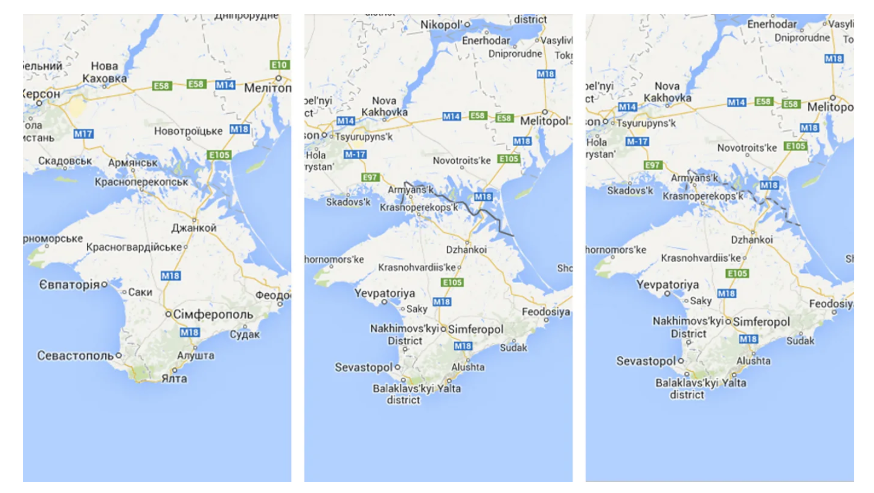
These three disparate cartographic representations signal the disputed nature of the border and also point to the sometimes-complicated intersection of cartography, geopolitics and technology within GIS, highlighting several truths. First, maps are not neutral, they don’t just show geography; they reflect political claims and governments care deeply about how maps portray their territory because that can legitimize or undermine sovereignty claims. Second, tech companies like Google, Apple and others must comply with local laws where they operate, and for example within India, companies must depict Kashmir as fully within India. If a single “global” version of a map were used, it would almost certainly offend one side of the disputed border, so a cartographic compromise is to use geolocation through IP address to determine what version of the map the user should see.

3. Virtual Boundaries

As evidenced in the text above, boundaries can be either natural or human-made. A special type of human-made boundary is a virtual boundary or geofence. A geofence is a digitally defined virtual boundary that triggers action(s) when a mobile device, vehicle or other sensor enters or exits the defined zone. They are created by specifying spatial geometry in a GIS—such as a buffer around a point location, a polygon representing a facility’s footprint, or a corridor along a transportation route. Geofences are widely applied in domains such as logistics (tracking fleet vehicles), marketing (sending location-based promotions to mobile users) and emergency management (issuing evacuation alerts to residents in hazard zones). Because these boundaries exist only in digital form, geofences exemplify the flexibility of virtual boundaries: they can be created, modified or removed instantaneously without altering the physical environment. At the same time, their effectiveness depends on accurate positioning technologies, such as GPS, cell and Wi-Fi networks. Implementation of these virtual boundaries also raises important concerns regarding privacy, surveillance and data governance.

4. Zones

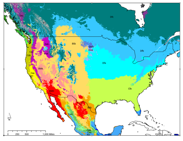
Boundaries and zones are related concepts. Boundaries represent the dividing lines or edges that separate different areas, or zones. Zones are areas that share common characteristics or attributes and are usually separated by boundaries. The concept of “zone” helps group regions with similar features together. Typically, zones are homogeneous areas defined by a specific criterion, such as land use, vegetation type, or risk level. Examples of zone types include land use zones, such as residential, commercial or industrial; climatic zones, such as temperate, tropical, polar; risk zones, such as flood zones, earthquake-prone zones, etc. (Figure 6).

5. Zonal Analysis

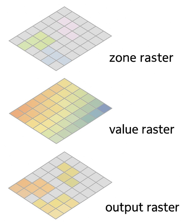
In GIS, a zone can be represented as either vector or raster data. In the vector format, a zone includes all features with the same attribute value (e.g., ZONE = residential). In the raster format, a zone refers to a set of cells or pixels in a raster with the same value. Zones can be of any shape or size and can be either contiguous or disaggregated. For datasets in the raster format, there is a set of tools collectively known as zonal analysis or zonal operations. Zonal analysis consists of computing an output using two input raster datasets—one with values of each cell and another with the zones. The input zone dataset defines the size, shape and location of each zone, whereas the input value dataset contains the values to be used in calculations for each zone. For example, we can use a raster dataset containing precipitation that fell over a 24-hour period during a heavy storm and combine it with a flood zone raster dataset to compute the average precipitation that fell over a 24-hour period in each flood zone. Zonal operations are similar to focal operations, where the zones themselves stand in place of neighborhoods (the shapes that are used for analysis in focal analysis operations) (Bolstad, 2019; Longley, 2005) (Figure 7).

When considering zones as analytical containers that shape how we measure, represent and interpret space, the Modifiable Areal Unit Problem (MAUP) must also be discussed. MAUP occurs when spatial analysis results change depending on how boundaries are drawn or how data are aggregated into zones. The two main effects of the MAUP are the scale effect, where changing the size of zones alters the results; and the zonation effect, where the configuration of boundaries, even at the same scale, changes results. We can observe the scale effect of the MAUP by creating a map of unemployment rates shown at the census tract level versus the county level, wherein larger zones smooth variability, and smaller zones reveal more local detail. We can observe the zonation effect of the MAUP by creating a map of land cover diversity metrics at the grid cell, watershed or county level. The MAUP highlights that boundaries and zones are not neutral containers—they shape results in zonal analysis and can change statistical outcomes, especially in cases of human created boundaries and zones. Sometimes, zones and boundaries can be manipulated to ensure a specific outcome, as is the case with gerrymandering. Gerrymandering is when voting district boundaries are drawn in a way that gives one political group an unfair advantage and is essentially a special type of manipulated zonal analysis because it involves manipulating zones (electoral districts) to alter outcomes and favor a specific candidate or political group.

Since the MAUP can never be fully eliminated, several techniques have been developed to cope with MAUP. Multi-scale or alternative zone analysis can help, because analyzing across spatial scales (census tract, zip code, county) or zoning schemes (school districts or watersheds) can show whether findings are robust. Using natural units (watersheds, street networks) where possible instead of arbitrary administrative units can also help. Many other techniques have been applied to counter the MAUP, including dasymetric mapping and areal interpolation, and others (Mennis, 2019).

6. Crisp vs. Fuzzy Membership

An important consideration regarding zones as an analytical concept relates to how zone membership is determined.  For many concepts, a binary classification applies, i.e., a feature or cell/pixel either is or is not a member of a zone. This is known as crisp membership—it is where membership in a single zone or category is assigned with absolute certainty. When crisp membership applies, a feature/cell/pixel either belongs to a zone (membership value = 1) or does not belong to a zone (membership value = 0). Crisp membership applies to land use classification, such as urban vs. rural; to cadastral mapping, such as property ownership; to political maps, i.e., within a specific country or outside of it, and many other concepts. However, there are some features that belong to categories with varying degrees of certainty. This is known as fuzzy membership—it is where membership values are continuous and range between 0 (no membership) and 1 (full membership). Fuzzy membership is best suited for situations with continuous classification or situations with gradual transitions. For continuous classification cases, features/cells/pixels can partially belong to multiple zones, and membership is expressed as a proportion or probability. For gradual transition cases, boundaries are not sharp but are defined by a gradient of membership, such as, for example, ecological zones or hazard risk zones (Burrough et al, 2015).

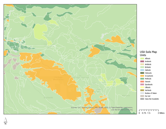
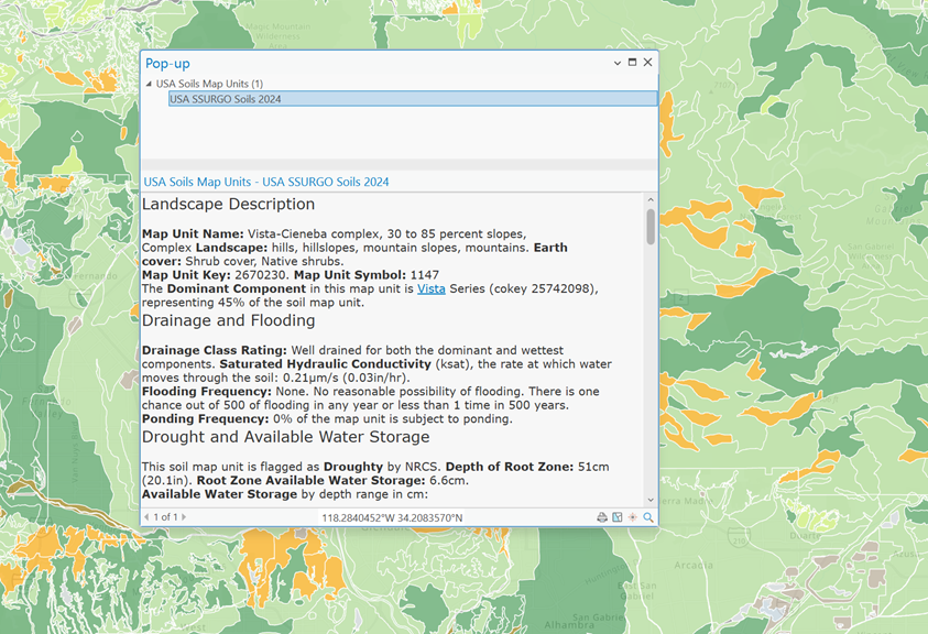
A notable example of using fuzzy membership for zones are soil maps in the United States, specifically the State Soil Geographic Database (STATSGO, now in its updated version STATSGO 2) and Soil Survey Geographic Database (SSURGO) soil classification schemes maintained by the US Department of Agriculture’s Natural Resources Conservation Service (USDA NRCS). Both STATSGO/STATSGO2 and SSURGO define map units (zones) not as a single uniform soil, but a collection of multiple soil components, each with an associate percentage composition. For example, a map unit or zone might be 60% sandy loam, 30% silty clay and 10% rock outcrop, where the percentage of each component can be considered a fuzzy membership grade (referring to the example above, a soil component that makes up 60% of a map unit or zone has a membership grade of 0.6, reflecting a stronger membership, whereas a soil component that makes of 10% of a map unit or zone has a membership grade of 0.1, reflecting a weaker membership). Thus, the soil map units or zones represent gradual transitions between soil types, acknowledge the uncertainty and heterogeneity, and reinforce the non-binary, fuzzy nature of soil classification. Soils are a great illustration or fuzzy set theory, where a location may partially belong to more than one class, and exact boundaries are not sharply defined (Burrough, 1989) (Figures 8 and 9).  

There are different methods of assigning fuzzy membership. In their 1996 paper titled “Fuzzy Representation of Geographical Boundaries in GIS,” Wang and Hall examine the “expressive inadequacy of the conventional vector boundary” and propose the use of fuzzy representation for geographical boundaries and describe four methods for determining fuzzy boundary membership (Wang and Hall, 1996). The four methods for assigning membership grades are: distance-based, based on the proximity of a location to a defined boundary; attribute-based, by evaluating the attributes of spatial features; statistical surface-based, in which statistical surfaces, such as probability density functions are utilized to model the uncertainty and variability of spatial phenomena; and expert knowledge-based, which incorporates expert judgement and domain knowledge to assign membership grades (Wang and Hall, 1996; Fisher, 2005).

7. Conclusion

Boundaries and zones are fundamental constructs in GIS, shaping how space is partitioned, represented, analyzed and understood. They can be natural or human-made, material or virtual, fixed or dynamic, crisp or fuzzy, and their delineation has profound implications for spatial analysis, scientific understanding and most importantly, decision-making. At their core, boundaries and zones act as analytical frameworks: they determine what is included or excluded, how phenomena are aggregated and how relationships across space are interpreted. Invariably, these frameworks are not neutral. From the challenges of the Modifiable Areal Unit Problem (MAUP) to the political stakes of disputed borders or gerrymandered electoral districts, boundaries and zones embody both technical and social choices. Recognizing the constructed and contingent nature of boundaries and zones and practicing techniques for minimizing negative impacts allows GIS practitioners to better interpret results, question assumptions and design more robust and transparent analyses.

References

- Bolstad, P. (2019). GIS Fundamentals: A First Text on Geographic Information Systems, 6th Edition. Acton, MA: XanEdu Publishing Inc.
- Burrough, P.A. (1989). Fuzzy Mathematical Methods for Soil Survey and Land Evaluation. European Journal of Soil Science 40(3), 477-492.
- Burrough, P.A., McDonnell, R.A., Lloyd, C.D. (2015). Principles of geographical information systems. Oxford University Press, USA.
- Chappell, B. (2014). “Google Maps Displays Crimean Border Differently in Russia, U.S.” National Public Radio.
- Fisher, P. F. (1999). Models of uncertainty in spatial data. Geographical Information Systems, 1, 191-205.
- Katz, C. G. (2022). “Why a Russian Invasion of Ukraine Would Be a Big Test for Google Maps.” TIME Magazine.
- Library of Congress (2025). The Disputed Area of Kashmir.
- Longley, P. A., Goodchild, M. F., Maguire, D. J., & Rhind, D. W. (2005). Geographic Information Systems and Science (2nd edition). Chichester: Wiley.
- Mennis, J. (2019). Problems of Scale and Zoning. The Geographic Information Science & Technology Body of Knowledge (1st Quarter 2019 Edition), John P. Wilson (Ed.).
- Miami-Dade County. (2025). GIS Data Hub.
- Ruggeri, A. (2014). The Politics of Making Maps. The BBC.
- United State Department of Agriculture (USDA) Natural Resources Conservation Service (NRCS). (n.d). Soil Survey Geographic Database (SSURGO).
- United State Department of Agriculture (USDA) Natural Resources Conservation Service (NRCS). (n.d). State Soil Geographic Database (STAGSGO2).
- Wang, F., & Hall, G. B. (1996). Fuzzy representation of geographical boundaries in GIS. International Journal of Geographical Information systems, 10(5), 573-590.
Learning outcomes
-
1946 - Define and differentiate the different types of boundaries and zones in GIS, including natural vs human-made, material or virtual, crisp or fuzzy, etc.
1947 - Explain the role of boundaries and zones in spatial analysis, including how they can influence analytical results.
1948 - Describe the key challenges associated with boundaries, such as the Modifiable Areal Unit Problem (MAUP), gerrymandering and disputed borders, and their implications for spatial analysis and map use.
1949 - Distinguish between crisp and fuzzy membership sets and use examples of geographic phenomena to demonstrate fuzzy membership for zones.
1950 - Apply boundary and zone classification to data (both raster and vector) from specific domain of study or research.