[FC-05-018] Adjacency and Connectivity

Richardson, H. N. and Curtin, K. M. (2026). Adjacency and Connectivity.  The Geographic Information Science & Technology Body of Knowledge (Issue 1, 2026 Edition).  John P. Wilson (ed.). DOI: 10.22224/gistbok/2026.1.4

1. Introduction
2. Connectivity in the Vector Data Model
3. Adjacency in Raster Analysis
4. Adjacency in Spatial Statistics
5. Other Uses of Adjacency and Connectivity

1. Introduction

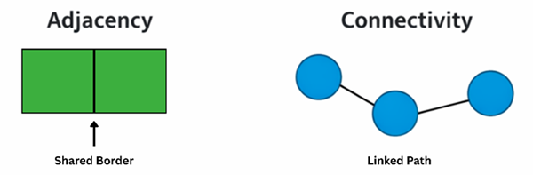
Adjacency and connectivity are foundational concepts in GIS because they define how spatial features relate through proximity and linkage. Together they represent fundamental spatial relationships that are central to understanding the organization and interaction of geographic features, and they provide a basis for modeling spatial dependence, movement, and interaction across geographic space. They underpin key analytical frameworks in raster analysis, vector data models, spatial statistics, and network analysis. Adjacency is defined as the condition in which two spatial entities share a common boundary or are immediately contiguous (Gold, 1989), whereas connectivity refers to the capacity of features to be linked through continuous paths or networks (Turnbull et al., 2018). These concepts are widely employed across geographic information systems (GIS), spatial statistics, urban and regional planning, transportation analysis, and environmental modeling. By quantifying and describing how spatial entities relate to one another, adjacency and connectivity provide essential insights into patterns of proximity, accessibility, and interaction within complex landscapes (Salleh & Ujang, 2023).

Critically, both adjacency and connectivity are topologically invariant properties, meaning that the relationships they describe are preserved under transformations such as stretching, scaling, or projection, provided the space remains contiguous (Deng & Revesz, 2001; Kumar, 2013). This invariance ensures that analyses based on these properties remain consistent even when spatial data are represented in different coordinate systems or at different resolutions (Salleh et al., 2021). However, processes that divide the space into separate components—such as the construction of barriers, fragmentation of habitats, or removal of network segments—can disrupt these relationships, altering previously adjacent or connected features. Such sensitivity highlights the importance of understanding both the structural and dynamic aspects of spatial topology when conducting rigorous spatial analyses.

From a methodological and analytical perspective, adjacency and connectivity underpin a wide range of computational and theoretical approaches in geography. In network analysis, connectivity governs the flow of resources, movement, or information, informing applications from transportation planning to hydrological modeling (Bunn et al., 2000; Liao et al., 2023). Adjacency is a critical component of raster-based spatial models, where interactions among neighboring cells drive processes such as diffusion, contagion, or habitat suitability assessments (Liang et al., 2024). The topological nature of these relationships allows them to be formally represented in graph-theoretic or matrix-based frameworks, enabling efficient computation of paths, clusters, and adjacency matrices (Osis & Donins, 2017). Consequently, adjacency and connectivity not only provide descriptive clarity but also support quantitative analysis and decision-making, facilitating the identification of bottlenecks, corridors, and areas of high spatial interaction.

2. Connectivity in the Vector Data Model

In early GIS data models, spatial features were primarily defined based on the adjacency or connectivity of points and the lines joining those points. The Dual Incidence Matrix Encoding (later renamed Dual Independent Map Encoding, or DIME) system, developed at the U.S. Bureau of the Census in the 1960s and 1970s, exemplifies this approach. DIME began with points as the fundamental spatial building blocks, each defined by precise coordinates such as latitude/longitude or x, y values (U.S. Census, n.d.). When these points were connected, the resulting lines were stored in a relational structure, capturing the connectivity of features. Further, when lines intersected or were incident to one another, those connections were recorded to define polygons. The primary goal of this encoding was to create unambiguous polygon definitions, as population statistics and demographic data collected by the Census Bureau needed to be accurately associated with polygonal spatial features such as census tracts, blocks, counties, and states (National Archives, 2025 February). By systematically encoding connectivity, the DIME system provided a rigorous and replicable method for defining complex spatial structures (U.S. Census, n.d).

Given that digital spatial data sets from the U.S. Bureau of the Census were among the first widely available, comprehensive, and freely distributed GIS layers, the DIME system, and its successor, the Topologically Integrated Geographic Encoding and Referencing (TIGER) system, became the dominant vector data models for decades. These models facilitated not only the creation of maps but also spatial analysis, routing, and demographic studies across the United States. Other vector-based GIS systems adopted similar approaches, emphasizing connectivity as the foundation for building accurate and topologically consistent polygon layers. By focusing on connectivity, these models ensured that adjacent features were represented consistently and that shared boundaries between polygons were recorded only once, reducing redundancy and enabling efficient storage and retrieval of spatial information (GISGeography, n.d.).

However, the strong focus on polygon-building based on connectivity imposed certain constraints on the vector data model. These models were necessarily planar: all features were treated as existing on a single two-dimensional plane. Whenever features crossed in this plane, a connection was assumed, which worked well for administrative boundaries and census polygons but introduced challenges when modeling networks or structures that are inherently non-planar. For example, overpasses, tunnels, and three-dimensional infrastructure cannot be accurately represented using purely planar connectivity rules, requiring non-planar vector data models that permit a more realistic representation of these features (Fohl et al., 1996).

The emphasis on connectivity in early vector data models has had a lasting influence on modern GIS analysis, particularly in the areas of network modeling and topological consistency. Contemporary applications, such as transportation routing, utility network management, and hydrological modeling, rely on the explicit representation of nodes and edges. By encoding the connections between spatial entities, GIS can calculate shortest paths, identify network bottlenecks, and simulate flow across complex systems. Furthermore, topological consistency ensures that shared boundaries and intersections are correctly represented, preventing errors in overlay analyses, spatial joins, and multi-layered data integration. In this way, the early focus on connectivity not only enabled the precise definition of polygonal features but also established the computational and theoretical foundation for the sophisticated network and topological analyses that are central to modern GIS practice (DiBiase et al., n.d.).

3. Adjacency in Raster Analysis

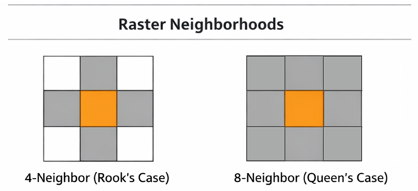
Although the early GIS use of adjacency and connectivity were focused on vector data models, adjacency is also a fundamental concept in raster-based GIS analysis, defining the spatial relationship between neighboring cells within a grid. In a raster dataset, each cell represents a discrete unit of space with a particular attribute value, and adjacency determines which cells are considered neighbors for analytical purposes. Common definitions include four-cell adjacency (rook’s case) and eight-cell adjacency (queen’s case), which influence how information propagates across the raster (rdrr.io, n.d). This concept is central to a wide range of raster-based analyses, including hydrological surface flow modeling, habitat suitability assessments, and landscape connectivity studies. By defining adjacency, analysts can systematically examine how local interactions between cells influence broader spatial patterns and processes (Turner, 2005).

Adjacency plays a critical role in modeling surface flow across raster landscapes. In hydrological analysis, for example, water movement is simulated by evaluating the relative elevation of neighboring cells and determining the direction of flow from each cell to its lowest adjacent neighbor. This approach relies on the adjacency relationships within the raster to construct flow direction and accumulation grids, which form the basis for delineating watersheds, stream networks, and flow paths (Barnes et al., 2014). Accurately capturing adjacency ensures that surface flow is represented realistically, reflecting the influence of topography on water movement and enabling robust modeling of erosion, runoff, and sediment transport (Singh, 2018).

In raster-based GIS analysis, smoothing techniques are used to reduce local variability and noise in raster datasets by leveraging adjacency relationships between neighboring cells. These techniques operate on defined neighborhoods (e.g., 3×3 windows) and modify cell values based on statistics computed from adjacent cells, effectively generalizing spatial patterns while mitigating small, isolated anomalies. For example, a low-pass or mean filter computes the average of surrounding cell values to smooth abrupt changes, reducing “salt-and-pepper” noise and highlighting broader spatial trends in continuous surfaces. Such filters are conceptually equivalent to applying a focal mean operation across adjacent cells and are commonly used in preprocessing elevation models or remotely sensed imagery to enhance visual and analytical quality (“Low pass filter smooths the data by reducing local variation…”) (Nasir, 2017). Beyond mean filtering, majority and boundary filters smooth discrete classified rasters by replacing a cell’s value with the most frequent class within its neighborhood or by expanding and contracting zones based on adjacent cell connectivity, which helps clean jagged zone edges (e.g., in land-cover maps) (Esri, 2025). More advanced methods such as edge-preserving anisotropic diffusion or median filtering can attenuate noise while retaining sharp transitions by accounting for local adjacency characteristics during smoothing (Nartiss, 2025). These adjacency-based smoothing approaches play a critical role in preparing raster data for subsequent analyses—such as flow modeling, segmentation, and classification—by balancing noise reduction with the preservation of meaningful spatial structure.

Beyond hydrology, adjacency relationships are integral to network and pathfinding analyses on raster surfaces, such as those employing Dijkstra’s algorithm. In this context, raster cells are treated as nodes in a graph, with adjacency defining the potential connections between nodes. Dijkstra’s algorithm then calculates the shortest or least-cost path from a source cell to a destination, taking into account the costs associated with moving between adjacent cells. This approach is widely applied in ecological modeling, route optimization, and hazard assessment, allowing analysts to identify optimal pathways across complex terrain (Medrano, 2021). By combining raster adjacency with cost-based metrics, GIS can represent spatial constraints, obstacles, and heterogeneous landscapes, providing a computationally efficient framework for spatial decision-making. The principles of adjacency in raster analysis, therefore, not only enable localized neighborhood operations but also underpin sophisticated surface flow modeling and network-based pathfinding, demonstrating its central role in spatial analysis and modeling.

4. Adjacency in Spatial Statistics

The use of adjacency in raster operations represents one type of analysis that depends on this sort of spatial relationship. Adjacency also provides the structural basis for analyzing spatial dependencies more generally, enabling statisticians to quantify how observations at one location relate to those at neighboring locations. In spatial statistical analysis, adjacency determines which units are considered “neighbors” for the purpose of measuring spatial autocorrelation, identifying clusters, or modeling dependencies. For example, in lattice-based analyses, adjacency matrices encode whether two polygons or raster cells share a common boundary (contiguity) or lie within a specified distance threshold (distance-based or k-nearest neighbor schemes). Such spatial weights representations are a standard component of spatial modeling (Cliff, 1981). These relationships are crucial in understanding how the value of one spatial unit may be influenced by or correlated with nearby units, thereby offering insight into spatial clustering, dispersion, and heterogeneity.

Although there are many ways to define a neighborhood for the purpose of testing for spatial dependence, adjacency is one of the most commonly used, for example, to calculate the spatial autocorrelation metrics such as Moran’s I and the Getis-Ord statistics. In Moran’s I, the spatial weight matrix encodes which units are considered neighbors, and this definition strongly affects the detection of clustering or dispersion (Negreiros et al., 2010). Local indicators of spatial association (LISA), which identify localized clustering patterns and hotspot detection methods, such as the Getis-Ord Gi* statistic, also rely explicitly on adjacency. A location is only identified as a statistically significant “hot spot” if it and its neighbors, as defined by the adjacency scheme, show consistently high values. This approach is widely used in fields such as crime analysis, disease mapping, and environmental monitoring (Chen, 2020).

Beyond exploratory measures, adjacency underpins more advanced spatial regression and econometric models. In spatial lag models, adjacency determines how outcomes in one unit are influenced by outcomes in neighboring units. In spatial error and conditional autoregressive (CAR) models, adjacency structures the correlations among residuals or random effects, allowing dependence to be explicitly modeled across space. Extensions include locally adaptive CAR models, which allow correlation strength to vary depending on the spatial contexts (Lee & Mitchell, 2012), and Bayesian models that estimate adjacency structures when they are uncertain (Gao & Bradley, 2019). Perhaps most notably, the suite of network-based spatial statistics developed over the past several decades reframes spatial dependence in terms of connectivity and distance measured along networks rather than across planar space, enabling point pattern analysis, clustering, and interaction tests that are intrinsically constrained by network structure. These methods provide the statistical foundation for analyzing events and processes that occur along roads, rivers, and other linear networks (Okabe & Sugihara, 2012; Okabe & Yamada, 2001).

Because adjacency structures encode the assumed pattern of spatial dependence, the choice of definition—whether contiguity, distance, or k-nearest neighbors—can greatly affect results. Analysts often perform sensitivity analyses to assess robustness to different adjacency schemes (Hwang, 2024). Properly defining adjacency is therefore essential to accurately capturing spatial dependencies and identifying meaningful patterns, from disease hotspots to socioeconomic clustering and ecological processes.

5. Other Uses of Adjacency and Connectivity

Adjacency and connectivity are not only theoretical constructs but also practical building blocks for reconstructing relational structures from spatial data. One common application in GIS and spatial analysis is generating networks from polygon centroids: adjacency matrices are constructed where each centroid becomes a node and connections between nodes reflect shared boundaries or nearest neighbor relationships, enabling quantitative analysis of spatial structure and interaction. This conversion from spatial geometry to graph representation underlies many regional and urban models where proximity influences flows and clustering.

In transport geography, adjacency look-ups and connectivity matrices are cornerstones of accessibility and movement analysis, with scholars emphasizing graph-based representations of transport systems to model flows, routing, and network performance across space. Street network studies formalize road intersections as nodes and street segments as edges, enabling formal optimization and connectivity analysis across infrastructures (Marshall et al., 2018).

Computational geometry techniques such as Voronoi (Thiessen) polygons and Delaunay triangulation explicitly encode adjacency and nearest neighbor relationships in spatial point sets. A Voronoi diagram partitions space into regions around each point that are closer to that point than to any other, making adjacency of Voronoi cells a natural descriptor of spatial nearness that can be used for neighbor analysis and influence zones. Its dual, the Delaunay triangulation, forms a triangulated mesh connecting points in a way that preserves proximity information and supports connectivity analyses in surface modeling, interpolation, and network construction (Sen, 2009).

These constructions have been applied in recent empirical research across diverse domains. For example, a 2025 study of architectural networks in traditional Tujia villages used Voronoi diagrams combined with graph theory to analyze spatial layout and connectivity patterns, demonstrating how Voronoi-derived adjacency informs cultural and ecological interpretations of spatial organization (Yang et al., 2025). Another recent uses complex network metrics calculated from adjacency matrices to explore the structure and evolution of national terrestrial adjacency networks, illustrating how topological properties (e.g., degree distribution, network density) reveal connectivity patterns at national scales (Zhi et al., 2024). Additionally, extensions of Delaunay triangulation methods have been proposed to generate synthetic networks that better capture local topological features in power grid and infrastructure systems, showing the broader applicability of geometric adjacency for realistic network modeling (Dey et al., 2023).

By working at the intersection of spatial geometry and network theory, these approaches operationalize Tobler’s First Law of Geography—“everything is related to everything else, but near things are more related than distant things”—such that adjacency becomes a quantifiable expression of nearness and connectivity in analytic models (Tobler, 1970).

Key References

• Anselin, L. (1988). Spatial Econometrics: Methods and Models.
• Cliff, A., & Ord, J. (1981). Spatial Processes: Models & Applications.
• Longley, P., Goodchild, M., Maguire, D., & Rhind, D. (2015). Geographic Information Systems and Science.
• O’Sullivan, D., & Unwin, D. (2010). Geographic Information Analysis.
• Turner, M. (2005). Landscape Ecology in Theory and Practice.

GIS Data Models and Topology

• U.S. Census Bureau. DIME and TIGER/Line technical documentation.
• Worboys, M., & Duckham, M. (2004). GIS: A Computing Perspective.

Raster and Network Analysis

• Barnes, R., Lehman, C., & Mulla, D. (2014). “Priority-Flood Algorithms for Flow.”
• QGIS / ArcGIS documentation for flow modeling and least-cost path tools.

ESRI Tools:

• Connectivity—ArcGIS Pro | Documentation
• Topology in ArcGIS—ArcGIS Pro | Documentation

QGIS Tools:

• https://docs.qgis.org/3.44/en/docs/training_manual/vector_analysis/network_analysis.html
• https://www.qgistutorials.com/en/docs/3/basic_network_analysis.html
• https://principles-and-applications-of-rs-and-gis.readthedocs.io/en/latest/network-analysis.html

References

- Barnes, R., Lehman, C., & Mulla, D. (2014). An Efficient Assignment of Drainage Direction Over Flat Surfaces in Raster Digital Elevation Models. Computers & Geosciences, 62, 128–135.
- Bunn, A. G., Urban, D. L., & Keitt, T. H. (2000). Landscape connectivity: A conservation application of graph theory. Journal of Environmental Management, 59(4), 265–278. Bunn, A. G., Urban, D. L., & Keitt, T. H. (2000). Landscape connectivity: A conservation application of graph theory. Journal of Environmental Management, 59(4), 265–278.
- Chen, Y. (2020). New framework of Getis-Ord’s indexes associating spatial autocorrelation with interaction. PLoS ONE, 15(7), e0236765.
- Cliff, A. D., & Ord, J. K. (1981). Spatial processes: models & applications (Vol. 44). London: Pion.
- Deng, Y., & Revesz, P. (2001). Spatial and topological data models. In Information modeling in the new millennium (pp. 360-382). IGI Global Scientific Publishing.
- Dey, A. K., Young, S. J., & Gel, Y. R. (2023). From Delaunay triangulation to topological data analysis: Generation of more realistic synthetic power grid networks. Journal of the Royal Statistical Society Series A: Statistics in Society, 186(3), 335–354.
- DiBiase, D., Baxter, R., King, B., Sloan, J., & Goldsberry, A. (n.d.). 3. Vector extracts from MAF/TIGER. The Nature of Geographic Information, Penn State College of Earth and Mineral Sciences
- Esri. (n.d.). Smoothing zone edges with Boundary Clean and Majority Filter. ArcGIS Pro 3.4 Documentation.
- Fohl, P., Curtin, K. M., Goodchild, M. F., & Church, R. L. (1996). A Non-Planar, Lane-Based Navigable Data Model for ITS. In M. J. Kraak & M. Molenaar (Eds.), International Symposium on Spatial Data Handling (Vol. 1, pp. 7B17-7B29). International Geographical Union.
- Gao, H., & Bradley, J. R. (2019). Bayesian analysis of areal data with unknown adjacencies using the stochastic edge mixed effects model. Spatial Statistics, 31, 100357.
- GIS Geography. (n.d.). A complete guide to TIGER GIS data.
- Gold, C. M. (1989). Spatial adjacency-a general approach. Proceedings of the Auto-Carto 1989, 298-312.
- Hwang, J. (2024). Alternative adjacency matrices and spatial analysis [Doctoral dissertation, Western Michigan University]. ScholarWorks at WMU.
- Kumar, N. P. (2013). A short note on the theory of perspective topology in GIS. Annals of GIS, 19(2), 123–128.
- Lee, D., & Mitchell, R. (2012). Locally adaptive spatial smoothing using conditional autoregressive models (No. arXiv:1205.3641). arXiv.
- Liang, Y., Zhu, J., Ye, W., & Gao, S. (2024). GeoAI-Enhanced Community Detection on Spatial Networks with Graph Deep Learning (No. arXiv:2411.15428). arXiv.
- Liao, C., Zhou, T., Xu, D., Cooper, M. G., Engwirda, D., Li, H.-Y., & Leung, L. R. (2023). Topological relationship-based flow direction modeling: Mesh-independent river networks representation. Journal of Advances in Modeling Earth Systems, 15, e2022MS003089.
- Marshall, S., Gil, J., Kropf, K., Tomko, M., & Figueiredo, L. (2018). Street Network Studies: From Networks to Models and their Representations. Networks and Spatial Economics, 18(3), 735–749.
- Medrano, F. A. (2021). Effects of raster terrain representation on GIS shortest path analysis. PLoS ONE, 16(4), e0250106.
- Nartiss, M. (2025, October 25). r.smooth.edgepreserve: Smoothing with anisotropic diffusion. GRASS GIS 8.6.0dev Documentation, GRASS Development Team.
- Nasir. (2017, October 23). Smoothing raster using ArcGIS Desktop? [Forum post]. Geographic Information Systems Stack Exchange.
- National Archives and Records Administration. (2025, February). Digital cartographic data holdings.
- Negreiros, J. G., Painho, M. T., Aguilar, F. J., & Aguilar, M. A. (2010). A comprehensive framework for exploratory spatial data analysis: Moran location and variance scatterplots. International Journal of Digital Earth, 3(2), 157–186.
- Okabe, A., & Sugihara, K. (2012). Spatial Analysis Along Networks: Statistical and Computational Methods. John Wiley and Sons.
- Okabe, A., & Yamada, I. (2001). The K-Function Method on a Network and Its Computational Implementation. Geographical Analysis, 33, 271-290.
- Osis, J., & Donins, U. (2017). Topological relationship. In Topological UML modeling: An improved approach for domain modeling and software development (pp. [xx–xx]). Elsevier Science.
- rdrr.io (n.d.). adjacent: Adjacent cells in raster: Geographic Data Analysis and Modeling. R Package Documentation.
- Salleh, S., & Ujang, U. (2023). Current uses of topology in 3D GIS: An overview. IOP Conference Series: Earth and Environmental Science, 1274, 012007.
- Salleh, S., Ujang, U., & Azri, S. (2021). 3D Topological Support in Spatial Databases: An Overview. The International Archives of the Photogrammetry, Remote Sensing and Spatial Information Sciences, XLVI-4/W5-2021, 473–478.
- Sen, Z. (2009). Spatial modeling principles in earth sciences (Vol. 10). Berlin/Heidelberg, Germany: Springer International Publishing.
- Singh, V. P. (2018). Hydrologic modeling: Progress and future directions. Geoscience Letters, 5(1), 15.
- Tobler, W. R. (1970). A Computer Movie Simulating Urban Growth in the Detroit Region. Economic Geography 46: 234–240.
- Turnbull, L., Hütt, M.-T., Ioannides, A. A., Kininmonth, S., Poeppl, R., Tockner, K., Bracken, L. J., Keesstra, S., Liu, L., Masselink, R., & Parsons, A. J. (2018). Connectivity and complex systems: Learning from a multi-disciplinary perspective. Applied Network Science, 3(1), 11.
- Turner, M. G. (2005). Landscape Ecology: What Is the State of the Science? Annual Review of Ecology, Evolution, and Systematics, 36(Volume 36, 2005), 319–344.
- United States Census Bureau. (n.d). Dual Independent Map Encoding. Last accessed April 13, 2026.
- Yang, J., Huang, Z., Zhao, A., Wu, X., Chen, Y., Hou, Q., & Lin, Z. (2025). Spatial network model and vitality optimization as illustrated by Chinese traditional Tujia villages. Npj Heritage Science, 13(1), 404.
- Zhi, Z., Liu, J., Liu, J., & Li, A. (2024). Geospatial Structure and Evolution Analysis of National Terrestrial Adjacency Network Based on Complex Network. Journal of Geovisualization and Spatial Analysis, 8(1), 12.
Learning outcomes
-
2015 - Define and distinguish between adjacency and connectivity as fundamental spatial relationships.
2016 - Explain why adjacency and connectivity are topologically invariant and why this matters for spatial analysis.
2017 - Identify how adjacency operates in raster analysis, including neighborhood definitions and focal operations.
2018 - Explain the role of adjacency in spatial statistics, including spatial autocorrelation and regression models.
2019 - Apply concepts of adjacency and connectivity to network analysis, pathfinding, and accessibility studies.
2020 - Evaluate how different definitions of adjacency influence analytical results and modeling outcomes.
Related topics
- [AM-02-006] Grid Operations and Map Algebra
- [AM-05-075] Intro to Network & Location Analyses
- [DM-01-028] Topological Relationships
- [FC-05-014] Directional Operations
- [FC-05-015] Shape
- [FC-05-017] Proximity and Distance Decay
Additional resources