[AM-09-088] Fuzzy Aggregation Operators

Zhu, A-X. (2024). Fuzzy Aggregation Operators.  The Geographic Information Science & Technology Body of Knowledge (2024 Version), John P. Wilson (Ed.). DOI: 10.22224/gistbok/2024.1.14

1. Introductory Concepts
2. Fuzzy Aggregation Operators
3. Application of Fuzzy Aggregations
4. Relevance to Geography

 

1. Introductory Concepts

1.1  The "Set" Concept

A set is a collection of distinct objects that share a unique list of properties. A set is a group, not an individual object. An individual object in a set is referred to as a member or an element of the set. The list of properties defining the set is used to evaluate the membership of an object in the set. 

An example of a set is the term “tall people”. It contains a group of people who are considered tall. Here the property used to evaluate the membership of person in “tall people” is the height of a person. How to define “tall” using height depends on which logic framework one adopts. There are basically two logic frameworks: Boolean (crisp) and Fuzzy.

1.2 Crisp set (Boolean logic)

A crisp or Boolean set is a set whose elements fully qualify for membership in the set. In other words, an object can either have full membership (100%) or no membership (0%) in the set, nothing between. “A crisp set is a set in which all members match the set concept, and the set boundaries are sharp” (Burrough and McDonnell, 1998, pp. 268).
For the “tall people” example, if one considers that a person 6 ft in height is tall, then everyone over 6 ft in height belongs to the “tall people” set and anyone below this height is not in this set at all. In this case, the cutoff is hard. The mathematical expression for the set of “tall people” is given in Equation 1:

Equation (1).   Tall people: if height > 6 ft  

One characteristic of Boolean set is that it is simple to understand and easy to implement. All what is needed is the cutoff value for the set. The other characteristic is that it assumes no variation among its members. For example, the Boolean set of “tall people” does not distinguish a member with a height of 6.8 ft from a member with a height of 6.1 ft. This second characteristic presents problems for describing geographic phenomena. For example, the concept of “deciduous forests” often contains individual forests with small portions of evergreen tree spices mixed in them. The level of this mixing is different from forest to forest and from location to location. The Boolean set of “deciduous forests” ideally only contains deciduous trees. However, in the real world, there are very few forests composed purely of deciduous trees. What we call “deciduous forests” is a set which is often composed of mainly deciduous trees. Using Boolean set to describe the concept of “deciduous forests” is somewhat inappropriate and misleading in this sense.

1.3 Fuzzy set (Fuzzy logic)

A fuzzy set is a set whose elements share the properties defined for the set at a certain degree which ranges from 0.0 to 1.0 with 0.0 meaning no membership in the set and 1.0 full membership, anything between expressing different levels of membership.

The notation of a fuzzy set often takes the form of an object and membership pair, such as  , where x is the object and  is the membership for x in fuzzy set  and  is the membership function for fuzzy set   (Burrough and McDonnell, 1998, p. 269).

The fuzzy set of "tall people" can be defined as below (Equation 2).

Equation 2: 

There are three parts within Equation 2: one for a person whose height is less or equal to 5 feet, who will have no membership in "tall people" at tall; the second part for a person whose height is between 5 and 6.5 feet, whose membership is computed using (x-5)/1.5; the third is for a person whose height is more than 6.5 feet, in this case the person has a membership of 1 (full membership) in "tall people". Given the above membership function for “tall people,” people with the following heights (in ft) (5, 5.6, 6.0, and 6.5 ft) will have the following respective memberships in the fuzzy set of “tall people”: [(5, 0.0); (5.6, 0.40); (6.0, 0.67); (6.5, 1.0)].

As can be seen above, one characteristic of a fuzzy set is that it does capture the variation in its members by assigning different levels of membership (belonging). This characteristic allows users, particularly users of geography, to express the varying nature of geographic features/phenomena, such as the varying proportion of evergreen species in the “deciduous forest” concept discussed earlier. The other characteristic of fuzzy set is the membership function , which is the key in defining a fuzzy set and demands much more knowledge from the subject field than what is needed for defining a Boolean set.

1.4 Fuzzy Membership and Membership Functions

There are two important notions we need to observe when using fuzzy set (fuzzy logic). First, fuzzy membership values are dependent on the membership function and one can define different membership functions for the same group of objects under different contexts. For example, for ordinary people, the above membership function for defining “tall people” would make good sense. However, for basketball players, the sense of “tall” is certainly different from our ordinary sense. A 6.0 ft person certainly can be considered tall in an ordinary sense but not necessarily tall among the basketball players of the NBA where the average is around 6.6 ft. All of these say that fuzzy membership functions can be very domain specific.

The second notation is that membership under fuzzy logic is mostly continuous (certainly depending on the nature of the application domain). Figure 1 below shows the membership gradation for “tall people” with regard to height of a person under the two contexts discussed above.

There are three basic forms of fuzzy membership functions which are often used in fuzzy mathematics (Figure 2): the bell-shaped, Z-shaped and S-shaped curves. The bell-shaped curve (function) describes that there is an optimal attribute value or range over which membership in the set is at unity (1.0) and as the attribute of the object deviates from this value or from this range the membership value decreases. For example, the concept of “moderate elevation areas” can be captured using this membership function.

The Z-shaped curve describes the scenario that there is a threshold value for the attribute of an object, smaller than which the membership is at unity (1.0) and greater than which the membership decreases. “Low elevation areas” can be expressed using this function (the lower the elevation values the higher the membership in the fuzzy set of “low elevation areas”).

The S-shaped curves define membership in opposite to that characterized by the Z-shaped curves. The concept of “high elevation areas” can be depicted using S-shaped membership function (the higher the elevations the higher the membership in the fuzzy set of “high elevation areas”).

 

If one examines these three types of membership functions closely, one will discover that the Z-shaped and the S-shaped membership functions are parts of the Bell-shaped curve. The Z-shaped is the right half of the bell-shaped curve with a membership value of 1 for the left half. The S-shaped is the left half of the bell-shaped curve with membership being 1 for the right half of it.

Given the above, the bell-shaped curve is often used as an example for explaining the metrics commonly used to define a membership function. As we have seen that a membership function for a fuzzy set describes how membership value changes with respect to changes of the attribute of objects. Thus, we must first choose a function which describes the general trend of gradation. For a bell-shaped curve, there can be many functions to achieve that shape (such as the Gaussian function or the normal distribution curve). Most of these functions require the following parameters as depicted in Figure 3.

 

Where x is the attribute value of an object (entity), x0 is the attribute value where membership is 1, often used to represent the central concept of the fuzzy set. D1 is the width between the lower crossover (the lower value of x where the membership value is at 0.5) and x0 , D2 is the width between the upper crossover (the upper value of x where the membership value is at 0.5) and x0 (see figure above). d is the sum of D1+D2. This function can be modified to represent the other two membership curves (Z-shaped and S-shaped) by setting the membership to one side of the optimal value to 1 (left for Z-shaped, right for S- shaped).

1.5 Fuzzy Membership Map

A fuzzy membership map is a manifestation of a fuzzy set over space. Assume that there is a soil type, say A, occurring over a given area, the fuzzy set of Soil Type A is the collection of membership values for respective locations over the area being Soil Type A. In other words, we can treat this collection as a map showing the membership value for every location belonging to Soil Type A (clearly, some of the locations would have zero membership because the soils at these locations are not Type A at all). This map is referred to as the fuzzy membership map of Soil Type A.

Figure 4 shows the fuzzy membership map for Soil Series Basco over the Pleasant Valley watershed in Wisconsin, USA. The brighter the tone the higher the membership in Basco soil series. As we have indicated above, some areas (such as the valley bottoms and the lower part of the slopes) have membership of 0 while other areas such as the ridge tops and upper slopes have high membership values. This indicates that the soil series Basco mainly occurs on ridge and upper slope areas and its membership values decrease when one moves down the slope. This gradation from upper slope to lower slope is realistic for soil spatial variation because soils do change over landscape gradually. This example also shows how fuzzy representation can capture the spatial gradation of geographic variation.

 

1.5 Fuzzy vs. Boolean

The key difference between crisp set and fuzzy set is that fuzzy set allows members to have different degrees of belonging while crips set does not. This means that variation among members is captured (expressed) under fuzzy set but it not under crisp (Boolean) set.

2. Fuzzy Aggregation Operators

Fuzzy aggregations are logic operations used to combine or aggregate two or more concepts (sets) into one using words such as AND, OR, or NOT under fuzzy logic. Clearly, these logic operations can also be implemented under Boolean logic. Below we will examine the fuzzy aggregations with comparison to their counterparts under the Boolean logic.

The fuzzy aggregations discussed here are of two types: the general ones and the specific ones. The general ones are operations which exist both under Boolean and fuzzy logic, such as AND, OR, NOT, while the specific ones only exist under fuzzy logic, such as α-cut or hardening.

2.1 General Fuzzy Aggregation Operators

AND, OR, and NOT are the three basic logic operations in this category. There are certainly other more complicated ones, which are beyond the scope of this discussion. Interested readers are referred to the references at the end of this entry for more discussion.

2.1.1  The Fuzzy AND

computes the intersection of the two or more fuzzy sets using the minimum of the individual membership values from the individual sets. Thus, sometimes, it is also referred to as the “fuzzy minimum operator”. For example, let’s say that the soil series, “Basco” occurs at the locations where the geology is “Jordan Sandstone” and the slope gradient is “<20%” (Figure 5). This statement describes where the location is suitable for soil type Basco to occur. As the statement suggested, “Basco” occurs on landscape where the geology is “Jordan Sandstone” and slope gradient is “<20%”. For a given location whether or not that location is suitable for Basco to occur can be decided by checking (evaluating) if the location is on “Jordan Sandstone” geology AND (at the same time) if the slope gradient at the location is “<20%”. In fact, “locations” on “Jordan Sandstone” is one fuzzy set and “locations” whose slope gradient is “<20%” is another fuzzy set. Based on the statement in Figure 5, “Locations” which are suitable for “Basco” to occur is a new set to be computed from the two individual sets through the use of the Fuzzy AND operator.

To examine the membership for every location in Soil Series “Basco” across a given study area using the fuzzy AND aggregation, we first need the memberships for the individual sets: the membership value for every location to be “Jordan Sandstone” and the membership for every location to be “<20%” in slope gradient. We then aggregate these membership values using the fuzzy AND operator to derive the final membership in Soil Series “Basco” which is defined by “locations on Jordan Sandstone and with slope gradient being <20%”. The fuzzy AND operator aggregates the individual membership values by taking the minimum of the individual membership values, thus it is also referred to as the fuzzy minimum operator.

To obtain the individual memberships, we need to define the membership function for each of these two sets. Since there is no fuzzy about whether a location is on “Jordan Sandstone” or not, we will say that if it is on “Jordan Sandstone”, the membership is 1, otherwise 0 (You might say that this is a Boolean function, yes, it is for this case because there is no fuzziness here). The membership function for slope gradient is “<20%” would require us to understand the context or the nature of the fuzzy set. Here we know that this definition of membership is under the context of Soil Series “Basco”. So the definition of membership function for slope gradient “<20%” must consider the influence of slope gradient on the development of soil type “Basco”, which requires the understanding of soil formation or pedology. This reflects the concept that fuzzy set is not applied in blind; rather it must be combined with domain knowledge (the knowledge of the application domain).

Given this, to define the membership function for the concept “slope gradient<20%”, we first need to determine the type of form for the membership function. Based on the discussion earlier, we can use the Z-shaped curve to capture “slope gradient<20%” (because the smaller the slope gradient the higher the membership in this set) and let’s use the simplest function as below to capture this:

Once we know what form the membership function takes, we now need to determine what and   should be. This would require some understanding on how slope gradient impacts the development of Soil Series “Basco”, which is often obtained from domain experts (soil scientists in this case). For the purpose of this illustration, let us assume that 20% is the breakpoint (crossover) with the membership of 0.5 for slope gradient being 20% in the context of the development of Soil Series “Basco”. When the slope gradient is less than 20%, the membership is greater than 0.5 (upper crossover). We also assume that the membership value reaches 1 if the slope gradient is 10% or less (which means we have no doubt that the soil of the location is absolutely Basco). With these, we now have the values for   and  with  being 10% (the central concept when membership reaches 1) and d being 2*(crossover – the central concept)=2*(20%-10%)=20%. Our membership function for “slope gradient <20%” is now given as:

Table 1 below gives us the membership values for the individual sets and the results from the fuzzy AND aggregation (often referred to as “the truth table). For Location 1, the fuzzy AND produces a 0 for Basco to occur which is reasonable because the Oneota geology prevents Basco to occur. This also applies to Location 3. However, Location 2 and Location 4 are both on Jordan geology so the fuzzy membership for Geology=Jordan is 1 but the “slope gradient <20%” membership varies depending on the value of the slope gradients. The fuzzy AND produces 0.25 and 0.6 for the final fuzzy set, respectively. 

Table 1. Truth Table for the Fuzzy AND for Soil Series Basco

Location	Conditions	Geology Component (= Jordan)	Slope Component (Slope < 20%)	Fuzzy AND Value
1	Geology = Oneonta, Slope = 25%	0	0.25	0
2	Geology = Jordan, Slope = 25%	1	0.25	0.25
3	Geology = Oneonta, Slope = 18%	0	0.6	0
4	Geology = Jordan, Slope = 18%	1	0.6	0.

Table 2 shows the result from the Boolean AND for Soil Series Basco. The clear distinction between the fuzzy AND operator and the Boolean AND operator can be made if one compares these two tables (Table 1 and Table 2). The Boolean truth table is very hard, which means that it is either 1 or 0, nothing between, while the fuzzy truth table produces grades. As a result, the slight possibility such as at Location 2 is not ignored or eliminated as was in the Boolean situation. At the same time, the possibility is neither exaggerated as for Location 4 in the Boolean situation.

Table 2. Truth Table for the Boolean AND for Soil Series Basco

Location	Conditions	Geology Component (= "Jordan")	Slope Component (Slope < 20%)	Final Value
1	Geology = Oneonta, Slope = 25%	0	0	0
2	Geology = Jordan, Slope = 25%	1	0	0
3	Geology = Oneonta, Slope = 18%	0	1	0
4	Geologoy = Jordan, Slope = 18%	1	2	2

Under the GIS context where we are interested in knowing the locations (in the form of a map) which are suitable for Basco to occur, we use these tables to assess at every location the suitability at which Basco develops by examining if the location meets the two conditions as stated in the AND operation. If we apply this process to every location in an area, we will obtain a membership map showing the suitability for Basco to develop for every location over the study area.

One must be aware that in this process, we did not observe the soil itself at the location we mapped. In fact, we used the relationships of soil type Basco to geology and slope conditions to predict or infer the suitability for Basco to develop at a given location. Clearly, this fuzzy AND aggregation process can be used to map other geographic distribution such as landslide susceptibility, habitat suitability, and crime risk.

2.1.2 The Fuzzy OR

The fuzzy OR operator computes the membership for the union of the combining fuzzy sets using the maximum values of the membership values in the combining sets. For this, it is sometimes also referred to as the “fuzzy maximum operator.” Let’s use the landslide susceptibility mapping as an example (Figure 6). The statement says that a location whose landslide susceptibility is high if either the location is on “Shale” geology OR the slope gradient is “steep” (>50%).

Like with the fuzzy AND, we need first to define the membership functions for the two combining sets: Geology is “Shale” and Slope is steep (exceeding 50%). For the same reason, let’s use the Boolean function for the geology part. For the slope gradient part, let’s use the S-shaped curve as the type of the curve (the “greater than” expression typically calls for the S-shaped curve). Given that we still use the simplest form as we used before, the membership form for the S-shaped curve is:

Let’s assume 50% is the lower crossover (that is the membership based on slope gradient is 0.5 at 50% of slope gradient and increases when the slope gradient increases), and further assume that the membership based on slope gradient to be 1 when the slope gradient reaches 80%. This gives us  being 80% and d being 60%, respectively. The membership function for slope exceeding 50% to be:

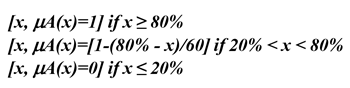
Table 3 below gives us the membership values for the individual sets and the results from the fuzzy OR aggregation of these two sets. Table 4 shows the truth table for this under the Boolean OR. The difference between the Fuzzy OR and the Boolean OR is clear.

Table 3. Fuzzy Truth Table for the Fuzzy OR Operator for Landslide Susceptibility

Location	Conditions	Geology Component (= "Shale")	Slope Component (Slope > 50%)	Final Value
1	Geology = Oneonta, Slope = 30%	0	0.17	0.17
2	Geology = Shale, Slope = 30%	1	0.17	1
3	Geology = Oneonta, Slope = 60%	0	0.67	0.67
4	Geology = Shale, Slope = 60%	1	0.67	1

Table 4. Truth Table for the Boolean OR

Location	Conditions	Geology Component (= "Shale")	Slope Component (Slope > 50%)	Final Value
1	Geology = Oneonta, Slope = 30%	0	0	0
2	Geology = Shale, Slope = 30%	1	0	1
3	Geology = Oneonta, Slope = 60%	0	1	1
4	Geology = Shale, Slope = 60%	1	1	1

 

2.1.3 The Fuzzy NOT

The fuzzy NOT operator computes the complement of a given fuzzy set. By complement, we mean that the operator subtracts the membership of an object in the given fuzzy set (original fuzzy set) from 1. In other words, a fuzzy NOT often produces the opposite of the set being negated. For example, the outcome for the set “the areas of not moderate elevation” can be produced by applying a “NOT operator” to the “areas of moderate elevation” defined using the bell-shaped curve. This will result in a membership function as depicted in Figure 7a. For comparison, the “NOT Moderate elevation” under the Boolean NOT is a step function as shown in Figure 7b.

 

2.2 Some Other Fuzzy Set Operators

2.2.1 The alpha-cut Operator

An α-cut is a process of selecting those members of a fuzzy set whose membership values is greater than a prescribed value (α). For example: select from the “total people” set the members with membership value above 0.8. This will produce a list of members whose membership is greater than 0.8 in “total people.”  The output from this operation is often a Boolean set. A different α value produces a different set. One can create multiple Boolean sets from a single fuzzy set by using different α values. One can also create a Boolean set by using two α’s, the upper one and the lower one.

As another example, select a group of people with membership value for “tall” is between 0.3 – 0.7, where the upper α is 0.7 and the lower α is 0.3.

α-cut is useful when you only have limited resources but want to maximize your coverage of the most vulnerable areas under a disaster relief scenario. If you have a fuzzy set of impacted areas with the degree representing the degree of damage, then you can use the α- cut to examine how far down from the most impacted to the least impacted areas you can cover with the resources you have.

2.2.2 The Hardening Operation

Hardening is a process of aggregating memberships for a given object in multiple fuzzy sets for the purpose of assigning the object into one of the Boolean sets based on these fuzzy sets. Let’s use soil mapping as an example to illustrate this. Assume that we have four soil types (A, B, C, D) in a given area. For any given location in the area, under fuzzy logic there are four membership values for that location each corresponding to membership in A, B, C, and D, respectively. What we now want is to assign a soil type (A, B, C or D) to this location for simplicity, how do we decide which soil type should be assigned to this location based on the membership values? The process converting these membership values of soil types into one soil type is a good illustration of “hardening”. People typically assign the soil type whose membership is the highest among the competing soil types to the location.

Hardening is widely used in creating a Boolean representation (map) of geographic variation from a group of fuzzy membership maps (See Section 1.2.3). Given that you have four types of soils: Basco, Council, Edmond, and Orion (the left part of Figure 8). Each has a membership map with light tone being the high membership in the corresponding soil type. For a single location, it has four different membership values (one for each class). Which class are we going to label the location as? The hardening process is the common approach used to achieve this by assigning the location with the label of the class whose membership value is the highest among the four. Let’s say for a location we have membership values in the four soil classes above as [0.3, 0.4, 0.1, 0.2], respective to the order of the soil types above. The hardening process will label that location as Council because the membership in Council at this location is the highest. Repeat this process at every location and we will produce a map of soil types with one location only assigned one of the four soil types (the right part of Figure 8).

How is hardening different from the fuzzy AND and fuzzy OR operations? First of all, it is not a logical operation. It is a conversion of fuzzy membership maps into a Boolean class map. It only applies to fuzzy membership maps. Second, it produces a class label for each location, not the membership value.

3. Application of Fuzzy Aggregations in Geography

3.1 Application Context

We use prediction of soil spatial variation (digital soil mapping) as an example to illustrate the application of fuzzy aggregations in geography. The details of this application can be found in (Zhu, 2006; 2008). By prediction we mean that we use the easily observable conditions from environmental variables related to soil development to predict (infer) the soil conditions (for simplicity soil class is used here as the condition) which are difficult to obtain directly (Zhu et al., 2001). In other words, we use the environmental conditions under which a given soil type occurs as surrogates to map soils.

The basic idea in achieving this prediction is to evaluate the similarity between the environmental conditions at an unvisited location and the environmental conditions for a given soil class. It is based on the premise that the more similar the environmental conditions at the location to these of the prescribed soil class, the higher the membership of the local soil at the location in the prescribed soil class (Zhu et al., 2018; Zhu, 2024). Thus, this similarity is taken as the membership of the environmental conditions at the candidate location belonging to the environmental conditions defined for the given soil class. If we take the environmental conditions defined for the given soil class as a set and the environmental conditions at a location as an object, then the prediction simply becomes evaluating the membership of an object in a set under fuzzy logic, a classic fuzzy aggregation problem. This fuzzy aggregation consisting of two major steps: determination of individual memberships based individual environmental conditions under fuzzy logic and aggregation of these individual memberships under fuzzy logic to obtain the final membership (the similarity) of the local soil in the prescribed soil class.

In order to accomplish this aggregation, we need two types of information that must be acquired first: environmental conditions at each location (a GIS database) and the knowledge on the environmental conditions for each soil class. The former is used to define the individual objects (locations) for which the membership values are to be determined and the latter is used to define the fuzzy membership functions of the soil classes.

3.2 Process of Digital Soil Mapping

The basic steps in digital soil mapping are: 1) Prepare GIS data layers on the environmental conditions for the given area, such as bedrock geology, slope gradient, elevation, and profile curvature in the above example; 2) Quantify the membership functions for each participating soil class (the fuzzy set); 3) Evaluate through fuzzy aggregation at each location the membership based on the quantified membership functions in each soil class; 4) Derive the soil type map for the area using hardening.

3.2.1 Compilation of GIS Data Layers on the Environmental Conditions (Predictors)

For soil mapping the predictors are often variables related to climate, topography, organism, parent materials (Zhu et al., 2001). Data on climate variables such as temperature and precipitation are readily available at weather stations. These weather stations data can be used to create data layers of temperature and precipitation using spatial interpolation techniques.

Variables on the terrain conditions often include elevation, slope gradient, slope aspect, profile curvature and planform curvature. Information on these variables can be derived using terrain analysis techniques. Organism information typically includes vegetation conditions which can be obtained from remote sensing techniques through image processing methods. Data on parent materials of soils can be obtained from a geological map (Zhu et al., 2001).

3.2.2 Quantification of Membership Functions for Soil Classes

To define the membership functions for each soil class, one needs the knowledge on under what typical environmental conditions each class occurs. Processes and techniques for acquiring this knowledge are beyond the scope of this entry. Interested readers are referred to Zhu (1999) for more details. Figure 9 shows this knowledge on the soils in a small watershed in Wisconsin, USA used in this example.

 

Let us use Soil Series Basco as an example to illustrate how to use the knowledge to define the membership functions. As Figure 10 shows the environmental conditions where Basco typically occurs. For Basco, we need four membership functions: one for “Jordan bedrock geology”, one for “slope gradient <20%”, one for “elevation greater than 950 ft”, and one for “profile curvature convex to linear”. The quantification of membership functions was discussed in the fuzzy membership function definition section earlier and the quantified membership functions for Basco under fuzzy logic is shown in Figure 10. ST in Geology means Jordan Sandstone.

 

The Boolean counterparts for the Basco soil as an example (Figure 10) are listed in Table 5.

Table 5. Boolean quantification of relationships

Conditions	True (1)	False (0)
Geology	If Jordan	Otherwise
Slope Gradient	< 20%	>= 20%
Elevation	> 950 feet	<= 950 feet
Profile Curvature	Convex to linear	Otherwise

 

3.2.3 Evaluation of Each Location Using the Quantified Membership Functions

With the membership functions defined, the membership for each location belonging to a particular soil class (here we used soil series) can be determined. The overall process of evaluation can be divided into two major steps (Figure 11) (using Soil Series Basco as example): The first step is to compute the individual membership value based on each environmental condition using the respective membership defined earlier and the second step is to compute the final membership of belonging to Basco by aggregating these sets using the fuzzy AND operator, based on the statements in the knowledge, “ Jordan bedrock geology AND slope gradient <20% AND elevation greater than 950 ft AND profile curvature convex to linear.”

 

If we do this evaluation for all locations in the area, we will get a map showing where Basco is, that is the membership map for Basco as we discussed earlier. This evaluation is done using the fuzzy AND aggregation because there are four conditions with each being a fuzzy set and linked with an “AND” operator. Figure 12 (left) shows the membership map for Basco in the Pleasant Valley area.

 

Figure 12 (right) shows the result from a Boolean AND aggregation based on the knowledge in Table 5. In this case each location will receive either 1 or 0 with 1 being Basco (all of these four conditions are met) and 0 not Basco (at least one of these conditions is not met). White colored areas are Basco and the black areas are non-Basco.

One can clearly see the differences between the results from the fuzzy AND aggregation (fuzzy mapping) (Figure 12 left) and that from the Boolean AND aggregation (crisp mapping) (Figure 12 right). The Boolean mapping expresses Basco at a location as 1 (it is) or 0 (it is not) while the fuzzy mapping expresses Basco at a location as a membership ranging from 0 to 1. With this presentation, spatial gradation of Basco over the area, particularly down the slope from the ridge, is clearly visible and this form of representation is more realistic than that based on the Boolean mapping.

We can apply the same process to predict the spatial distribution of the other three soil types. This will produce a total of four fuzzy membership maps (Basco, Elkmound, Council, and Orion). Each of the maps represents the similarity of the local soil to that soil type across the study area.

3.2.4 Derivation of the Soil Type Map

Once we have these membership maps, we have for each location four membership values (one for Basco, one for Elkmond, one for Council, and one for Orion). To create a map showing the different soil types over the area, we need to assign each location a soil class to form a Boolean map. This calls for the hardening process we discussed earlier, which assigns a location the soil type whose membership value is the highest among the competing soil types.

3.3 Characteristics of Mapping Through Fuzzy Aggregation

The characteristics of mapping geographic variation through fuzzy aggregation can be understood through comparison with the Boolean mapping. Boolean mapping is the common mapping paradigm most people adopt in geographic mapping. Figure 13 compares the results from these two types of mapping paradigms.

The first difference is that the Boolean map has holes in it while the fuzzy map does not. This is the result of the rigid evaluation under the Boolean logic. Due to the rigidness of the Boolean evaluation the conditions at some of the locations in the area do not meet all of the conditions specified for these soil types in the area. As a result, these areas are not assigned to any class. Typically, these unsigned locations are in the transitional areas between soil types. This means that under Boolean evaluation the soils in transitional areas can be completely missed out. On the contrary, fuzzy evaluation retains different levels of membership in a class and this level (grade) of membership along with memberships in other classes can be used to determine which class the location should be assigned to even through local conditions at the location do not fully meet the conditions of any soil type. This means that the fuzzy logic is much more flexible than the Boolean logic.

Another advantage of fuzzy aggregation is that the hardening process can also produce uncertainty information associated with assigning a location a soil class to which the soil at the location does not fully belong (Zhu 1997). Figure 14 shows the uncertainty map associated with the soil map in Figure 13 (left). The level of whitening in a color for a location indicates the level of uncertainty in assigning the local soil to the given class (representing by the color) (Burt et al., 2011). It is clearly shown that the highest level of whitening in colors are in the transitional areas where no soil classes were assigned in Figure 13 (right). Uncertainty in this regard cannot be produced under the Boolean aggregation.

 

4. Relevance to Geography

So far, we have discussed the basic aspects of fuzzy aggregation in comparison with its Boolean counterpart. The relevance of fuzzy aggregation to geography can also be highlighted through the comparison between the semantics behind fuzzy aggregation with that behind its counterpart with which we are so familiar.

4.1 Occurrence vs. Similarity

Occurrence is often used to refer to whether an event occurs or not. More than often, we assign some value to it to indicate how likely it is to happen. For example, we often hear weather broadcasters saying that “there is 95% chance it will rain.” It must be made clear here that the statement never addresses the nature of the rain (intensity and duration). It only concerns the occurrence (whether it happens or not). The value 95% is assigned to express the likelihood that it will occur.

Similarity on the other hand expresses the degree to which one thing (object) belongs or is similar to a predefined class or prototype or a known object. For example, one might say “Michael Douglas looks almost exactly like his father, Kurt Douglas”. This statement expresses the similarity of Michael Douglas to Kurt Douglas. It concerns the nature of being like Kurt Douglas, not whether Kurt Douglas would occur or not.

In a geographic sense, when we map soil (or any other geographic object/entities) over space using some prescribed classes, we are really saying how similar the object/entity at a given location is to those prescribed classes. We are not saying whether any of the prescribed classes will occur at that location because the soil does exist at that location already and we want to know how it compares to the prototypes (the prescribed classes) we already know. Therefore, for describing spatial variation of geographic objects/entities using a prescribed set of classes, the semantics behind similarity is more suited.

4.2 Probability vs Possibility

Probability deals with the chance that something will happen, and it is a measure of occurrence while possibility is a measure of similarity. The following examples are confusing, but the process of clarifying them is a way to illuminate the difference between probability and possibility and the relevance of fuzzy aggregation to geography.

Example 1:  “It is probable that we can have another passenger on the bus” expresses the chance of someone coming to take the bus while “It is possible that we can have another passenger on the bus” states whether the bus can hold another passenger, stating the similarity of the bus to full.

Example 2:  “There is a little chance that it will rain” is a probability statement saying if it will rain or not tomorrow. It says nothing about the intensity of the rain. The statement “It will rain a little” is a possibility statement expressing the intensity of rain, which is little.

4.3 Fuzzy Logic (Probability) vs. Boolean Logic (Possibility)

Boolean logic is for representing probability while fuzzy logic is for possibility. In the sense of classification, possibility is more appropriate because the object is already in existence, and we simply determine which class it is similar to. Examine the following two sentences and see which one makes more sense in geography.

• “The soil at this site is about 70% similar to the prototype of Miami Silt Loam.”
• “The Miami Silt Loam will occur at this location at 70%.”

Clearly, the first is more appropriate in geography because the soil already exists at that site. The question is the nature of what it is.

In classification, we want to know which class the local soil belongs to by comparing the properties of the local soil with those of the candidate classes. It is not the issue about which of the prescribed classes occurs at the given site. Classification is based on possibility, not probability. It is inappropriate to use probability to measure possibility even though we have been doing it for a long time and are very much used to the idea. It might be the time to conceptually change this habit, and to use possibility for classification.

4.4 Nature of Geographic Variation and Fuzzy Aggregation

By nature, geographic phenomena vary over space often gradually and prescribed classes (prototypes of classes) only exist in very limited locations. As a result, geographic phenomena at vast majority of locations are between types. Mapping these in-between type entities using predefined classes, which is often the case in geographic analysis, would naturally call for the application of fuzzy logic so that details of the in-between nature of geographic phenomena are not lost.

References

- Burrough, P. A. and McDonnell, R. (1998). Principles of Geographical Information Systems, 2nd Edition. Oxford: Oxford University Press.
- Burt, J.E., Zhu, A. X., Harrower, M. (2011). Depicting classification uncertainty using perception-based color models. Annals of GIS, 17(3), 147-153.
- Zhu, A. X. (1999). A personal construct-based knowledge acquisition process for natural resource mapping using GIS. International Journal of Geographic Information Science, 13(2), 119-141.
- Zhu, A. X. (2006). Fuzzy logic models in soil science. In Sabine Grunwald and Mary E. Collins (eds.), Environmental Soil-Landscape Modeling: Geographic Information Technologies and Pedometrics. New York: CRC/Taylor & Francis. pp. 215-239.
- Zhu, A. X. (2008). Rule based mapping. In: J.P. Wilson and A.S. Fotheringham (eds.), The Handbook of Geographic Information Science. Malden, MA: Blackwell, Malden. pp. 273-291.
- Zhu, A. X. (2024). Laws of Geography. In International Encyclopedia of Geography (eds D. Richardson, N. Castree, M.F. Goodchild, A. Kobayashi, W. Liu and R.A. Marston). Wiley Online Library.
- Zhu, A. X., Hudson, B., Burt, J., Lubich, K., & Simonson, D. (2001). Soil Mapping Using GIS, Expert Knowledge, and Fuzzy Logic. Soil Science Society of America Journal, 65(5), 1463-1472.
- Zhu, A. X., Lu, G., Liu, J., Qin, C. J., and Zhou, C. (2018). Spatial prediction based on the Third Law of Geography. Annals of GIS, 24(4):225–240.
- Zhu, A.X. (1997). Measuring uncertainty in class assignment for natural resource maps using a similarity model. Photogrammetric Engineering & Remote Sensing, 63, 1195-1202.
Learning outcomes
-
66 - Compare and contrast Boolean and fuzzy logical operations
Compare and contrast Boolean and fuzzy logical operations
395 - Describe fuzzy aggregation operators
Describe fuzzy aggregation operators
971 - Exemplify one use of fuzzy aggregation operators
Exemplify one use of fuzzy aggregation operators
1730 - Explain the concept of set and its relationship to membership functions and fuzzy aggregation.
Explain the concept of set and its relationship to membership functions and fuzzy aggregation.