[CP-03-021] Social Networks

Andris, C. (2019). Social Networks. The Geographic Information Science & Technology Body of Knowledge (2nd Quarter 2019 Edition), John P. Wilson (Ed.). DOI: 10.22224/gistbok/2019.2.9.

1. Definitions
2. What is a social network?
3. Components and characteristics
4. Metrics of importance/distinction
5. Connections with geography and GIScience
6. Data sources and software

1. Definitions

social network: a configuration of individuals (nodes) and their relationship to other individuals
node or vertex: an entity that typically represents an individual or, less commonly, a group of individuals (e.g. an institution)
edge, link or arc: a connection between entities that represents a relationship
friends, ties: a node’s relationship or connections (edges)
network or graph: configuration of nodes attached by edges
node features: attributes or characteristics ascribed to nodes
edge weight: a parameter that describes the strength or cost of connection
modules or communities: mathematically-detected groups of nodes that are better connected to their own group than to an external group

2. What is a social network?

Interpersonal relationships are a common phenomenon in our lives, these include friendships, work colleagues and schoolmates, family, online acquaintances, and romantic ties. These are often collectively referred to as “friends”, or if the social network of a particular individual is in focus, “ego” (the individual) and “alters” (the ego’s friends)-called an egocentric network. The collection of relationships can be modeled as a network in order to understand dynamics like, who bridges the network together, how people are linked to friends of friends, and how many connections certain people have.

Social Networks (SN’s) have roots in sociology, specifically from Durkheim and Simmel, who studied the relationships between individuals, as well as researchers who collected data about relationships in the 1910s and 1920s (Freeman 1996). The first visualized network schema, called a sociogram (Figure 1), is attributed to Jacob Moreno (1934). Since, SNs have been used to understand human behavior, such as examining how information spreads, whether there are ‘popular’ or central people, and how people form cliques and groups. Some famous social networks include “toy” networks such as that of Florentine (Italy) marriages (Padgett & Ansell, 1993) or Les Miserables character connections (Knuth 1993). More pragmatic network analyses have shown clear racial homophily (a tendency to connect to someone with similar characteristics) between high school friends (Moody 2002), or the group formation in a network of a karate club (Zachary, 1977), visualized below (Figure 1).

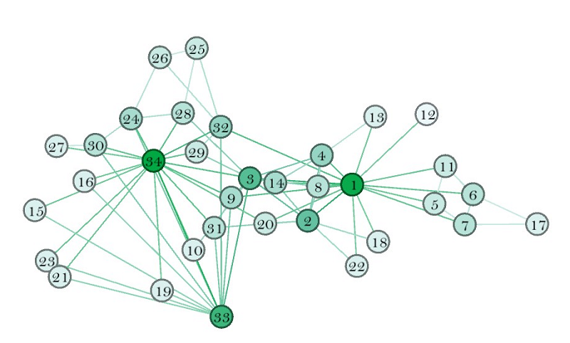
Figure 1: A classic social network example is that of a karate club in the 1970s, where each individual (node) is coded with a number and an edge exists between the nodes if they report high levels of interaction. Each node is colored based on their “degree”, i.e. the number of friends they have. Dark green nodes (1, 2, 34 and 33) have the most network friends. Node 12 has the fewest network friends. This graphic was made in Gephi. Source: author. 

3. Components and characteristics

3.1 Components

Networks consist of nodes and edges. In GIS, levels of measurement (e.g. nominal, ordinal, continuous (interval/ratio), binary and fuzzy), are key for understanding the variables that spatial entities can take on. The same kinds of distinctions apply to social network connection data.

Node Features
Features ascribed to nodes are most often nominal or categorical. When there are two types (e.g. teacher and student) this is called a bipartite network. When there are multiple types (e.g. 12 different military ranks), these can be distinguished using a block model. Otherwise, nodes in a social network are typically referred to by a name, or ID number, to preserve anonymity. The number of connections a node has is called its degree (K).

Edge Features
Features ascribed to edges, often called edge weights, can be nominal, ordinal, or continuous data. A binary or an unweighted network (0/1) records the presence or absence of a tie between two people. This is good for fast computation, but it's not always helpful for social science inquiry, because interactions are coded the same for, say, someone's spouse as for their dentist. Or for someone who plays both roles! A variation on binary networks is a signed network (ex. -1, 0, 1) describing whether an individual has a positive, negative or no relationship with another. Edges can be coded with:

• The nature of a relationship, such as professional, kin (family), friends, romantic, classmate, acquaintance, etc.
• The rank of one’s relationships from strongest tie (rank 1) to weakest tie.
• The strength of the relationship (ex. 1-100 where 100 is the strongest).
• Contact or visitation frequency (weekly, bi-monthly, etc.).**
• Telecommunications frequency (number of phone calls/SMS, social media likes, e-mail, etc.)
• Whether the edge connects people of similar or different features (age group, or same race).

Edges that are coded with multiple values are known in the social network community as multigraphs. Edges also have directionality, which occurs when a respondent A connects to individual B, and B does not connect to A in return. In a directional network, nodes can have an in-degree (K_i) and out-degree (K_o) that counts their incoming and outgoing connections, respectively.

3.2 Network measurements

Network dispersion (i.e. between nodes) is measured in hops, an integer value that reflects how many edges need to be traversed to reach another node. The diameter of a network is defined as the longest shortest path, i.e. the distance (in hops) between the nodes that are most dispersed in the network.  Network density is calculated as the number of existing edges / number of total possible edges between all nodes. The density ranges from 0-1. A network with density of 0 is rare, and not particularly helpful; but would theoretically consist of unconnected individuals--called isolates. Conversely, a clique is defined as a fully connected network, where all nodes are connected to all other nodes.

Networks are often characterized by their degree distributions, a histogram or probability density function of the number of nodes that exhibit a certain degree. Social networks differ from other types of networks (e.g. road networks or computer networks) because they usually have central members, and are built by a process known as preferential attachment, where new nodes tend to attach to nodes that already have a high degree. As a result, the degree distribution of social networks has few nodes with high degrees, some nodes with mid-range degrees, and many nodes with low degrees.  

Nodes are also split into groups, subgraphs, modules, etc. using community detection algorithms (ex. Girvan & Newman, 2002). These indicate what kinds of natural groupings form within the network by mathematically (and iteratively) defining groups that connect internally to their given group more often than to nodes in another group.

4. Metrics of importance/distinction

Which nodes play important roles in the system? If these nodes were removed, there may be significant changes to the network.

4.1 Centrality

There are multiple types of centrality. Three popular metrics are degree centrality, closeness centrality, and betweenness centrality. Degree centrality is given as a node’s degree (K) divided by the total number of nodes in the network (N). Betweenness centrality is given as the number of times that a node (n_i) is used in a shortest path between all nodes in the network (n_ij). Closeness centrality is given as the average number of hops it takes a node (n_i) to reach all other nodes (n_j).  Betweenness and closeness centrality can be calculated for edges as well as nodes. Nodes can be measured by their eccentricity, the maximum shortest path to reach the farthest node in the network. Those with max(eccentricity) are said to be on the periphery of a network, vs. and those with min(eccentricity) are said to be in the central part of a network.

4.2 Embeddedness

To what extent is node embedded in the network? The clustering coefficient is a common way of measuring node embeddedness. The clustering coefficient is given as the number of connections between a node’s (n_i) friends (E_jk), divided by the total possible connections between them (K*(K-1)). In addition, nodes can be calculated as brokers, liaisons, etc. if they connect different configurations of disconnected friends (Freeman, 1977). Core/periphery models also exist to distinguish groups of nodes that comprise a center vs. those that lie on the outskirts of the network.

5. Connections with geography and GIScience

5.1 Geographic distance

Close distance between nodes (i.e. being nearby) tends to be linked to more ties, in a process called propinquity (Fischer, 1982). In addition to degree distributions, social network analysts produce distance distributions: frequency charts of the number of times an edge of a certain distance appears in a social network. It is almost always the case that the frequency of ties decay with increased distance. The rate in which they do so can be ascertained by these types of graphs. These distributions most often use Euclidean distance and can be enhanced by using GIScience calculations of travel time and cost between the two entities.

Metrics that balance distance and network hops or expanse can explain whether geographic nearness between nodes indicates connectivity. The route factor, is defined as the ratio of the number of hops between nodes in a social network to the Euclidean distance between the nodes (see O’Sullivan 2015). Each network has an average route factor. A newer metric, the network flattening ratio is defined as the ratio of the total (sum) distance of a network’s edges to the total distance that would preserve the degree distribution, but would minimize total edge distance (Sarkar et al., 2019). The purpose of these metrics is to compare the actual expanse of a network (how spread out it is over geographic space) with the traversability of the network-how easily different nodes can be reached. Moreover, a more traditional GIS spatial statistic, Moran’s I, can be used on both social networks and spatial extent to examine whether clusters in the network correspond to clusters in geographic space (Emch et al., 2012).

5.2 Place and nodes

Nodes often have place names as features (i.e. characteristics). If these are not assigned a priori, a spatial join of the node to (nearest) place point, or place polygon can be performed. For example, a student in a neighborhood may be assigned to her nearest elementary school, and the name of here elementary school may become a feature of her node. Or, a neighbor’s node may fall within the boundaries of the city of London, and so his node has a feature “London”. These features can be used to assess whether nodes with similar features are likely to be connected, or if they play similar roles in the network. For instance, perhaps individuals living on military bases (place = military base) are likely to be part of larger kinship social networks than the typical individual. Assigning platial features to nodes is subject to the same conflicting place name decisions as general GIS place-labeling or spatial joining exercises, and so these decisions should be made carefully.

5.3 GIScience and social networks

Social networks are able to be embedded into GISystems, given that nodes are geolocatable. Edges linking nodes can be visualized and sometimes spatially joined to the underlying spatial data. Traditionally the most common way of geolocating nodes is by their administrative or self-volunteered location (such as household location (Figure 2) zip code, workplace, etc.), although other options such as ‘real-time location’ or ‘activity space’ are viable options. A geolocated SN may span several continents or could be confined to one small street. A geolocated SN can then be integrated with spatial variables such as land use, agriculture, or access to points of interest like schools or places of worship (Faust et al. 2000).  

Theoretically, a geolocated social network embodies (aspects of) geographical and social relationships within a single structure. In its most basic form, this network reveals the extent to which ties are (geographically) nearby and to which nearby nodes are ties. The former indicates the extent of travel that is needed to meet, and the latter suggests the extent to which nodes have cultivated a local community—key aspects for understanding how relationships are configured in the landscape.

In computer and information science communities, geolocated social networks are often referred to as location-based social networks (LBSNs), a type of big data. LBSNs are passively-collected social data derived from social media sources such as Facebook, or call data records (CDRs), that often have millions of nodes and links (see Zheng, 2011). LBSNs can be easily collected without surveys or interviews: the node’s GPS or mobile phone traces are used to pin an individual to an activity space, and set of trajectories. LBSNs provide records on the individual’s spatial whereabouts and digital interactions (e.g. text messages or IMs) (Leskovec & Horvitz, 2014), making it easy for researchers to detect replicable patterns about social interaction and interaction frequency with nearby and distant ties. However, LBSNs lack information on the nature of a relationship (e.g. family or friend?), are unable to capture all of a node’s ties, and are limited to data on the medium’s users (e.g. Instagram users), and should be approached with these shortcomings in mind.

Figure 2. A geolocated social network of households in the Amazon where edges represent hosting one another at the home (courtesy of Paul Hooper) is divided into three modules. The households are then mapped atop a spatial image of the study area to show that nearer households tend to be in the same modules (from Andris, 2016). Source: author. 

6. Data sources and software

6.1 Example data sources

Limited data sources are available because social networks tend to lack geolocation information, however the following sources may be of interest.

• SNAP: Location-based Online Social Networks
• American Social Fabric Survey
• The Network Data Repository with Interactive Graph Analytics and Visualization
• Reality Mining: Sensing Complex Social Systems
• Nang Rong (Thailand) Project

6.2 Software

Available software is likely to change as different packages emerge and others retire. However, the following packages have been prominent in the network analysis community. (Note this is not an exhaustive list).

• UCINET: Borgatti, S., Everett, M., & Freeman L. (2002). UCINET 6 for Windows: Software for Social Network Analysis. Lexington, KY: Analytical Technologies.
• PAJEK: Batagelj V., & Mrvar A. (2003). Pajek: Analysis and visualization of large networks. In: Jünger M, Mutzel P, editors. Graph Drawing Software. New York: Springer. pp. 77–103.
• GEPHI: Bastian, M., Heymann, S., & Jacomy, M. (2009). Gephi: an open source software for exploring and manipulating networks. ICWSM, 8, 361-362.
• iGRAPH: Csardi, G., & Nepusz, T. (2006). The igraph software package for complex network research. InterJournal, Complex Systems, 1695(5), 1-9.
• **Colocation frequencies are key for geography because data is often collected geolocated from devices or self-report, and because the results illustrate the relationship’s demand to meet (i.e. colocate).

Further recommended reading

Hanneman, R., & Riddle, M. (2005). Introduction to Social Network Methods. Riverside, CA:  University of California, Riverside. Available online: http://faculty.ucr.edu/~hanneman/ 

Sarkar, D., Sieber, R., & Sengupta, R. (2016). GIScience considerations in spatial social networks. In International Conference on Geographic Information Science. pp. 85-98. Cham: Springer.

References

- Andris, C. (2016). Integrating social network data into GISystems. International Journal of Geographical Information Science 30(10): 2009-2031.
- Emch, M., Root, E. D., Giebultowicz, S., Ali, M., Perez-Heydrich, C., & Yunus, M. (2012). Integration of Spatial and Social Network Analysis in Disease Transmission Studies. Annals of the Association of American Geographers, 102(5), 1004-1015.
- Faust, K., Entwisle, B., Rindfuss, R. R., Walsh, S. J., & Sawangdee, Y. (2000). Spatial arrangement of social and economic networks among villages in Nang Rong District, Thailand. Social Networks, 21(4), 311-337.
- Fischer, C. (1982). To Dwell Among Friends. Chicago: University of Chicago Press.
- Freeman, L. C. (1996). Some antecedents of social network analysis. Connections, 19(1), 39-42.
- Girvan, M., & Newman, M. E. (2002). Community structure in social and biological networks. Proceedings of the National Academy of Sciences, 99(12), 7821-7826.
- Knuth, D. (1993). The Stanford GraphBase: A Platform for Combinatorial Computing. Reading, MA: Addison-Wesley.
- Leskovec, J., & Horvitz, E. (2014). Geospatial Structure of a Planetary-Scale Social Network. IEEE Transactions on Computational Social Systems, 1(3), 156-163.
- Moody, J. (2001). Race, School Integration, and Friendship Segregation in America. American Journal of Sociology, 107(3), 679-716.
- Moreno, J. (1934). Who Shall Survive?: A New Approach to the Problem of Human Interrelations. Washington, DC: Nervous and Mental Disease Publishing Co.
- O’Sullivan, D. (2014). Spatial Network Analysis. In: Fischer, M., Nijkamp, P. (eds) Handbook of Regional Science. Springer, Berlin, Heidelberg.
- Padgett, J., & Ansell, C. (1993). Robust action and the rise of the Medici, 1400-1434. American Journal of Sociology, 98(6), 1259-1319.
- Sarkar, D., Andris, C., Chapman, C. A., & Sengupta, R. (2019). Metrics for characterizing network structure and node importance in Spatial Social Networks. International Journal of Geographical Information Science, 33(5) 1017-1039.
- Zachary, W. (1977). An Information Flow Model for Conflict and Fission in Small Groups. Journal of Anthropological Research, 33(4), 452-473.
- Zheng, Y. (2011). Location-Based Social Networks: Users. In: Zheng, Y., Zhou, X. (eds) Computing with Spatial Trajectories. Springer, New York, NY.
Learning outcomes
-
613 - Describe the purpose of a social network and what it can reveal about relationships.
Describe the purpose of a social network and what it can reveal about relationships.
675 - Describe what nodes and edges represent, and the variables that can be ascribed to each.
Describe what nodes and edges represent, and the variables that can be ascribed to each.
1002 - Explain how a social network might interact with the built environment.
Explain how a social network might interact with the built environment.
1017 - Explain how different metrics reveal the 'importance' of nodes or edges in a social network.
Explain how different metrics reveal the 'importance' of nodes or edges in a social network.
1427 - List different properties that are used to describe an entire network.
List different properties that are used to describe an entire network.
1546 - Report on how a social network can have spatial properties.
Report on how a social network can have spatial properties.
Additional resources