[CV-04-031] Flow Maps

Steiner, E. (2019). Flow Maps. The Geographic Information Science & Technology Body of Knowledge (4th Quarter 2019 Edition), John P. Wilson (ed.). DOI: 10.22224/gistbok/2019.4.10. 

1. Definitions
2. A Brief History of Flow Maps
3. Categorizing Flow Maps
4. Design Considerations
5. Production Methods

 

1. Definitions

continuous flow map: a type of map that depicts the movement of phenomena on a continuous surface, where the flow can be measured at any point (e.g., wind); also called called “unit vector” flow maps

distributive flow map: a type of map that depicts phenomena being distributed between nodes (e.g., exports from a country) in a geographic network

edge: a vector path connecting two nodes

graph: a configuration of nodes and edges, as in a network graph

network flow map: the classic flow map type showing a series of locations joined by lines representing paths of travel (often straight lines) of varying thicknesses indicating the volume of flow on each segment of the network

node: an origin or destination in a flow map or graph

origin-destination (O-D) matrix: a matrix of origins and destinations indicating the volume of flow between each O-D pair

radial flow map: a single source distributive flow map with flow radiating out from the origin

Sankey diagram: a type of non-cartographic flow diagram that depicts the volume of flow through a system with proportionally-sized arrows

space-time path: a multidimensional graphic (often cubic) showing the path of an object – usually a person – through space over time; also referred to as “time-space” path

topology: the non-metric spatial relationship (e.g., connected) between nodes

 

2. A Brief History of Flow Maps

While the symbolic use of an arrow is thought to be less than four hundred years old (Finkel 2015), cartographers have long been interested in representing movement on maps, especially for maritime purposes.

2.1 Early Depictions of Flow (pre-1800)

Wind roses appeared on maps as early as the 13th century, but even before this the earliest illustrations that might arguably qualify as flow maps are those depicting rivers and streams. The basic method of symbolizing rivers—apparent even on ancient maps—is that of showing thin tapered lines joining successively wider lines before eventually emptying into oceans (Figure 1). These depictions appear realistic but are often more symbolic: they typically far exaggerate river widths and could be interpreted as illustrating flow volume rather than actual width. Such distortions are likely due to the outsized role of rivers in early transportation systems, and as such, these maps are quite effective at articulating general fluvial connectivity despite often obvious inaccuracies in river geometries – a characteristic we will see is typical of later flow maps.

 

Figure 1. Fluvial cartography has long symbolized river flow using tapered lines of varying widths. Source: G. H. Colton, 1861, via the David Rumsey Map Collection.

 

More explicitly symbolic depictions of flow did not appear on maps until the 17th century, when arrows indicating the direction of streamflow first appeared. The use of lines to demarcate the routes of explorers or military movements also became common in this era (Figures 2 and 3).

 

Figure 2. Maps from the late 17th century to early 20th century (left) commonly indicated stream flow direction with a single decorative arrow (de Fer, 1688; source: David Rumsey Map Collection). Dashed lines and dates plot the detailed path of Captain James Cook’s explorations of the Bering Strait. Note the use of two dash styles to indicate different years. Source: Cook, 1785, via the David Rumsey Map Collection.

 

Figure 3. Military maps documenting battle maneuvers were some of the first to characterize approximate flow with sweeping arrows, a technique that remains common today. Examples here include a Revolutionary War map of Huberton,Vermont (left) (Faden, 1780; source: David Rumsey Map Collection) and a hand-drawn map of the day’s action at Gettysburg (right). Source: Sneden, 1863, via the Library of Congress.

 

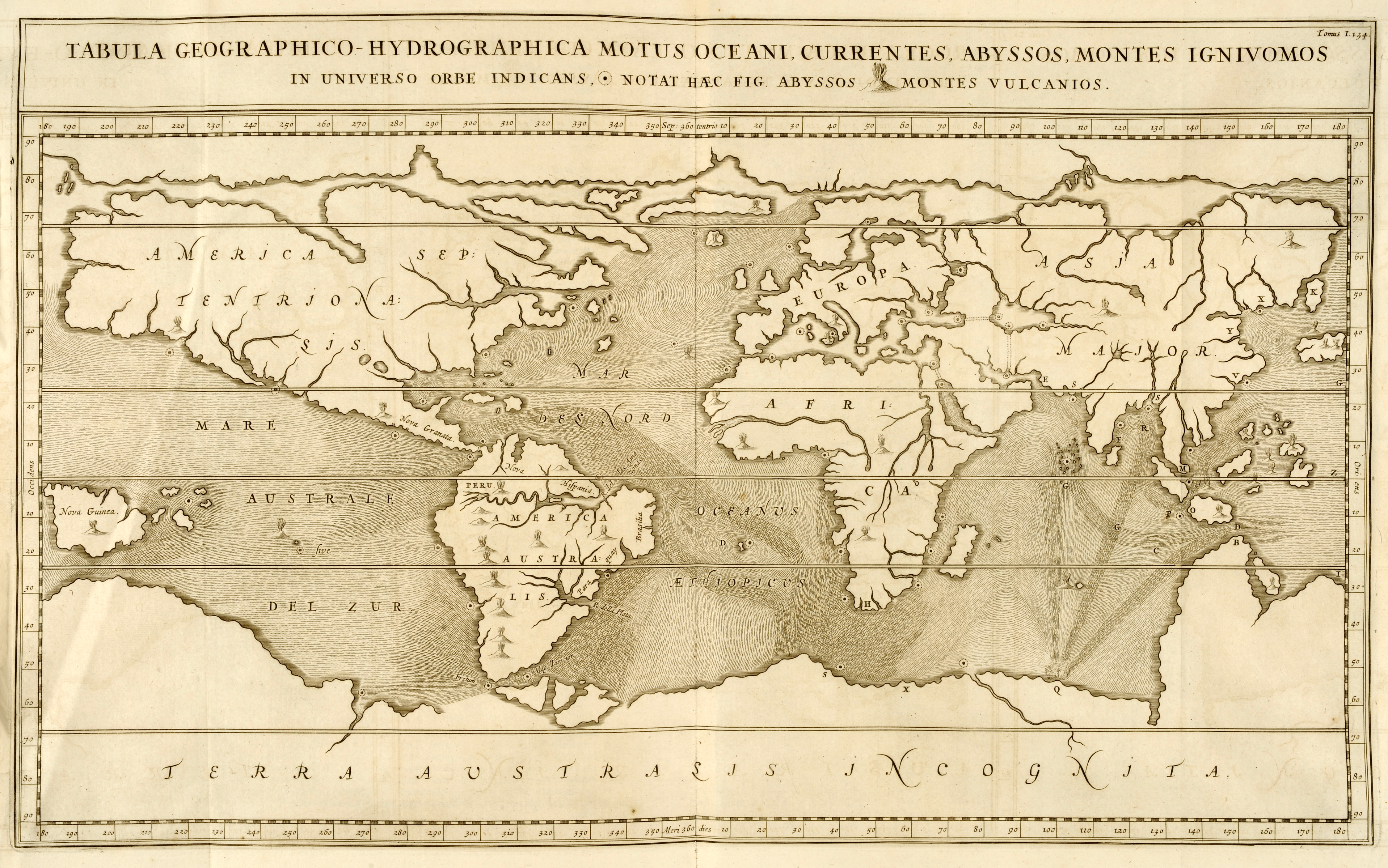
Meanwhile, maritime cartographers had been advancing parallel techniques for symbolizing observations of wind and water dynamics. Three of the most sophisticated early flow maps (and thematic maps more generally) of this style are displayed below (Figure 4). By this point, engravers had been using similar techniques with varying stroke length, width, and density to illustrate dynamic natural features (e.g., light, water, and clouds) for centuries, but none had applied the methods to communicate scientific observations in this way.

 

Figure 4. Athanasius Kircher’s 1665 map of ocean currents (top), Happel’s map of ocean “ebb and flow” (1685) and Halley’s trade wind map (1686) are some of the earliest examples of thematic flow maps. Halley was one of the first to symbolize flow direction with tapered strokes or tails. He explains: “I could think of no better way to design the course of the Winds on the Mapp,” although it stands to reason that the insight may have stemmed from his astronomical observations of a certain comet a few years earlier (1682). 

 

2.2 Thematic Maps Emerge

It was not until the early 1800s after William Playfair’s innovations in statistical graphics – in particular his advancement of the concept of proportional symbols (see Common Thematic Map Types) – that the classic form of thematic map showing volume of movement emerged. The earliest example of such a map is thought to be that of Henry Drury Harness in the Irish Railway Commission Atlas of 1837 (Harness, 1837) depicting the relative traffic volume on railways and ships throughout Ireland (Figure 5).

Figure 5. Arthur Robinson wrote that Harness’ 1837 maps “qualify as one of the more remarkable sets of maps ever made.” (Robinson, 1955). He also included the first dasymetric population density map in the same publication. Source: University College Dublin. 

 

Harness’s insight was to combine Playfair’s proportional scaling methods with a simplified illustration of a railway network. His map stands today as exemplary, as it employs several of the essential qualities of modern network flow maps, and the style has remained essentially unimproved since its invention.

Following Harness, Charles Joseph Minard employed a similar technique in the mid-19th century including his well-known 1869 diagram of Napoleon’s march on Russia as well as several other maps (e.g., exports of French wine, immigration, coal). Minard’s world maps are notable for their careful distortion of underlying geography without sacrificing intelligibility. Note in Figure 6, the Strait of Gibraltar is wide enough to accommodate the arrow showing the growth of the Egyptian cotton trade at its maximum scale in 1865.

Figure 6. Minard’s series of mid-19th century maps are the most well-known early examples of flow maps. He expertly combined quantitative and qualitative flow data, distorted underlying geographies, and elegantly illustrated branching and merging flow paths. Source: Minard, 1866, via the Library of Congress.

 

2.3 Modern Developments

Flow map developments since the 19th century have come in response to the rise of new infrastructural and technological networks – including automobile and air travel, communications, and energy. Numerous examples of transit mapping in the last century reinforce the value and stability of the basic technique. The canonical airline map (Figure 7), meanwhile, is a simpler variation, typically showing great circle arcs connecting origin and destination cities without an indication of traffic volume.

Figure 7. Air France developed a series of attractive maps of their routes beginning in the 1930s. Early versions used only straight lines; the need to accommodate the expanding flight availability seems to have led to the adoption of curved lines, which also had the advantage of adding a three-dimensional effect (Boucher, 1961; Source: David Rumsey Map Collection).

 

Meanwhile, non-cartographic methods for visualizing flow also arguably emerged with technological developments and the need to visualize these complex systems. The Sankey diagram, for example, was developed in the late 1800s to illustrate the thermal efficiency of steam engines, with variable width lines indicating the proportional amounts of energy flowing through parts of the system.

Figure 8. Sankey diagrams are often used to show magnitude of flow in and out of systems such as energy or material. This 2012 graphic shows the process of transformation of raw wood into paper products, recycled material, energy, and waste. Source: Van Ewijk et al., 2017.

 

More recently, other graphical treatments in the same vein as Sankey diagrams have developed, including alluvial diagrams (Figure 9) and circle migration plots (Figure 10). These plots share the same basic data structure of an origin-destination (O-D) matrix and the graphical concept of connecting a series of origins and destinations (nodes) with lines of varying thicknesses (edges).

The “node-edge” terminology used here draws from the parlance of graph theory in mathematics that is commonly used in network analysis – a graphical method that has proliferated in recent years along with the pervasion of social networking technologies. Of course, many network diagrams do not reflect geography at all but instead social connections or other relationships, but the same visual methods are applied.

 

Figure 9. Alluvial diagrams are sometimes described as Sankey diagrams. Typically they are read left-to-right and illustrate the changing composition of groups across multiple states or over time. While the above example does not include this feature, the “streams” often merge or branch as they move left to right to communicate the union or division of one or more groups. Source: Aisch, 2014; used with permission. 

 

Figure 10. Circle migration plots (also called circular flow plots) illustrate volume of flow between a fixed matrix of origins and destinations. Less commonly, flow is shown in both directions. Source: Abel, 2018; used with permission.

 

3. Categorizing Flow Maps

There is no clear consensus on a strict flow map typology as their styles and purposes are diverse and overlapping, and their subjects range from geographic to abstract. Thus, it is worthwhile for the reader to be familiar with a range of terms applied to flow maps.

Drawing from nearly a century’s worth of flow maps appearing in American text books, Parks (1987) described three key types:

• Network flow maps illustrate flow in a network between several origins and destinations. This term describes the classic flow map type with a series of geographic locations joined by lines representing paths of travel, often showing magnitude and direction of flow. These diagrams often (but not always) show an abstracted or highly generalized geography where the topology of the network is emphasized over the precise distances or paths between the nodes. The term also adequately applies to maps of transportation, communications, or energy networks where flow volume might not be directly depicted but flow potential would be central to the purpose of the map (as in airline and transit maps where routes are commonly shown as generalized curves to give the impression of flow).
• Radial flow maps illustrate flow from one source to many destinations or vice versa. This is essentially a simple network flow map that typically shows flow volume in one direction, either into or out of a single point.
• Distributive flow maps are a special type of radial flow map in which flows branch as they move from a single origin to many destinations or vice versa. While not strictly showing single origins, many of Minard’s 19th century flow maps employed this merging and branching method where branches are presumed to symbolize the partial disposition of shipments to multiple destinations along similar shipping routes.

Slocum (2009) did not distinguish the above types, but instead differentiated between maps showing migration of people (or goods) and continuous flows. Continuous flow maps (also called “unit vector” flow maps) are visually distinctive from the other types, depicting the magnitude and direction of flow of a phenomenon over a continuous surface. The term continuous here refers to the idea that the direction and magnitude of a flow can be observed or estimated at any point on the data surface.

Historically, continuous flow maps employed what might be called the “starry night” technique (after Van Gogh’s “The Starry Night”) where flow magnitude and direction is indicated by a series of parallel brush strokes (Figure 4). The method is also one of the few that can also effectively illustrate turbulence. With the aid of animation, standard raster techniques for surface representation (e.g., heat maps) have become the defacto technique to show continuous flow data (e.g., wind speed on a weather map) with flow direction illustrated with the aid of animation. Meanwhile, animation and computational algorithms have also revived the use of the “starry night” technique, employed beautifully in these recent illustrations of wind and ocean currents.

Other continuous flow methods include the use of abstract symbols at points indicating observations of magnitude and direction (e.g., wind arrows) or the use of a vector field where each cell of a regular or variable density grid is given a vector arrow indicating force and direction.

While not explicitly noted by Parks or Slocum, maps that indicate travel paths inherently express movement and should be noted, particularly given their near ubiquitous use with GPS devices for aiding navigation or tracking activity. This type of map typically depicts the movement of one or more objects (e.g., person, vehicle) between an origin and destination over time, representing a potential or completed journey. Multiple or complex paths inhibit interpretability, but can be aided by the addition of color, value, or transparency (Figure 11).

 

Figure 11. Continuous GPS collar tracking on migratory elk in the Greater Yellowstone Ecosystem illustrates the annual journeys and regional footprint of seven distinct elk herds. The use of color distinguishes the different herds and value/saturation represents time. © 2018 University of Wyoming and University of Oregon. Source: Wild Migrations: Atlas of Wyoming’s Ungulates. Oregon State University Press. Cartography: University of Oregon InfoGraphics Lab. 
 

Space-time paths are a special form of travel path maps that integrate time on a vertical axis in an attempt to distinguish between the speed and distance of travel (Hagerstrand, 1970). Figure 12 illustrates a unique and early example; more recently, 3D space-time cubes have been used to compare daily travel activities of people in urban settings (e.g., commute to work) (Kwan, 1999).

Figure 12: A unique example of a space-time path flow map illustrating the sequence of plays of a football game. Space is represented on the horizontal axis while time is portrayed vertically. Reproduced from original Boston Globe illustration by Brinton, 1919.

The term flow map might generally be understood also to include a class of graphs, charts, and diagrams that share similar design features to the origin-destination types described above, but are distinguished by their non-geographic layout. As previously noted, network diagrams, Sankey diagrams, alluvial diagrams, and circle migration plots are visually similar to flow maps and can be used to represent geographic data. Short of including line graphs and bar charts in this category, the purpose of many graphs is to show entities changing over time or in attribute and thus draw from the same symbolic palette (e.g., slope graphs, parallel coordinate plots, stream graphs and bump charts).

Given this broad diversity of origin-destination graphics, Gu et al. (2017) propose a comprehensive classification, with a focus on the visibility of origins and destinations and the use of qualitative and quantitative attribute data. Their classification matrix combining these dimensions reaches 30 possible types although they only identify real-world examples for half of them.

A final novel approach to consider for classifying flow maps would be as follows (Figure 13). Consider two orthogonal axes, one representing the spatial continuity (point, area, surface) and another representing the relative independence of the movement or flow (distinct to interdependent). Spatial continuity refers to how spatially complete the phenomenon is: only occurring at point locations vs. occurring everywhere (e.g., Cabelas stores vs.  air quality). Distinct movements generally refer to the movement or growth of a single object or set of discrete objects that do not significantly affect one another (e.g., commutes to work). Interdependent flows refer to the dynamic properties of an interconnected system where movement in one part of the system affects the other parts (e.g., ecosystems).

Figure 13. A typology of flow maps differentiated by the conceptual model of the phenomenon being mapped, along two axes: on the vertical axis, the range of spatial continuity from discrete points to continuous surfaces and on the horizontal axis, the degree of complexity. In this model, simple, isolated and distinct movements or spatial changes are contrasted with complex systems of dynamic flows with high degree of interdependence. The examples here suggest appropriate map symbology choices for the different conceptual models. Flow origin, magnitude, path, and direction have slightly different meanings depending on the type, and thus the map symbology is chosen to match how the phenomenon is conceived and the intended interpretation. Source: author.

 

4. Design Considerations

As flow maps serve diverse purposes and production remains poorly automated, there are numerous aesthetic and design considerations for cartographers to balance. Figure 14 summarizes the key considerations for vector flow map symbology.

Figure 14. Summary of design alternatives for representing different components of flow maps. Source: author. 

 

4.1 Generalization and Abstraction

Representing a large number of true geographic flow paths often produces visual complexity that might inhibit the general interpretability of a map. A common feature of flow maps is the abstraction of the flow geometry and/or geographic base map in order to emphasize the topological connections between origins and destinations and accommodate their aesthetic arrangement (see Scale & Generalization). Abstracted lines are most dramatic on network flow maps where the topology of the network is more salient than the precise path shapes (e.g., metro maps). Path smoothing and algorithmic clustering can also effective to reduce complexity in large flow datasets (Guo & Zhu, 2014).

A fundamental choice of the overall layout (see Visual Hierarchy & Layout) or projection (see Map Projections) is also important. As noted, there are a variety of non-geographic layout options to consider. If a geographic layout is chosen, thought should be given to the choice of projection (e.g., equidistant projection centered on single origin) and on the degree of generalization or distortion of the underlying geography. Carefully distorted base geography allows the cartographer to more effectively arrange flow paths without obscuring parts of the map or other flow paths.

4.2 Dynamic Flow Maps

Animation has become a common method for representing movement and flow (see Spatiotemporal Representation). These methods introduce several new considerations:

Flow direction

• animated paths revealing lines from origin to destination
• discrete objects moving along the path (possibly both directions)
• use of fading or “trails” to show previous time frames

Flow magnitude

• similar to static maps, depicted by line width, color, value, or transparency
• option of an accumulative presentation over time

Flow rate

• animated paths repeating or pulsing at varying rates
• density and speed of discrete objects moving along the path

4.3 Recommendations

There is little cognitive research that examines the interpretation of flow maps, so their design principles rely heavily on expert intuition (Jenny et al., 2016). Jenny at al. sought to address these issues in their user study of static origin-destination flow maps, reaching the following conclusions (Figure 15):

• number of flow overlaps should be minimized
• sharp bends and excessively asymmetric flows should be avoided
• acute intersection angles should be avoided
• flows must not pass under unconnected nodes
• flows should be radially arranged around nodes
• quantity is best represented by scaled flow width
• flow direction is best indicated with arrowheads
• arrowheads should be scaled with flow width, but arrowheads for thin flows should be enlarged
• overlaps between arrowheads and flows should be avoided

Figure 15. Jenny et al. identify the preferred flow line geometries and arrangements from a controlled user study. Source: author, after Jenny et al. (2016).

 

A question Jenny et al. did not consider is whether the perception of flow magnitude is affected by path length. A high-volume flow over a long distance occupies significantly more visual weight on an image than a flow of the same volume over a short distance, thus introducing a distorting effect on the impression of magnitude.

These recommendations also do not address several types of flow maps identified above: continuous flow maps, maps with merging or branching arrows, or maps with paths that closely follow geographic features (e.g., rivers). The design principles for these types of maps are not clearly established, so they rely on the judgment of the cartographer.

4.4 Summary of design recommendations

In summary. the key visual elements that make a good flow map include:

• Clear illustration of origins, destinations, and flow direction
• Representative line scaling that accurately reflects the relative volume of movement
• Judicious use of arrow heads so as to not overwhelm or distort the impression of volume
• Use of branching or merging flow paths where appropriate to reduce clutter
• Visually pleasing flow paths without awkward overlaps or intersections
• Appropriate use of generalization and/or distortion for flow curves and underlying geography

 

5. Production Methods

Several computerized methods have been attempted to facilitate the production of vector flow maps, but the style remains resistant to satisfactory automation. Good flow maps are typically hand-crafted affairs, prepared with the help of cartographic software (e.g., ArcGIS) but then heavily modified with a graphics package (e.g., Adobe Illustrator).

Tobler (1987) was the first to develop automated flow mapping software. Although by today’s standards the maps produced by Tobler’s software were rather crude (Figure 15), his algorithm was effective at highlighting dominant flows and modifying flow paths to pass through intermediate waypoints.

Flow map layout software developed by Stanford computer scientists (Phan et al., 2005) sought to improve on Tobler’s work to help solve the problem of visualizing networks. Their software focused on single-source flows and was effective at minimizing overlapping paths and supported branching/hierarchical flow structures (edge bundling). Buchin et al. (2011) improved on Phan’s work, demonstrating an algorithm (based on “Steiner trees”) that produces visually-appealing layouts with obstacle avoidance and no crossings. Similarly, Nöllenburg & Wolff (2011) created an effective method for generating attractive metro map layouts. These advances by the computational geometry community are promising, but the integration of these functions into commonly available software is limited.

 

Figure 15. Thirty years of automated flow mapping algorithms. Source: author.

 

Dedicated functions for flow mapping in GIS software have developed more slowly, although multiple options are now available:

• Network flow maps can be generated straightforwardly from carefully segmented geometry and line-width scaling (e.g., for traffic counts)
• Great circle or straight line paths for airline-type maps can be generated using the XY to Line function and then scaled according to a variable (Akella, 2011).
• Distributive Flow Lines Tool is a downloadable ArcGIS tool that creates branching paths roughly in the style of Minard’s maps.
• Canvas Flow Map Layer is a layer plugin for the ArcGIS Javascript API that creates dynamic Bezier curve-based flow maps.

References

- Abel, G. J. (2018). Estimates of Global Bilateral Migration Flows by Gender between 1960 and 2015. International Migration Review.
- Aisch, G., Geveloff, R. and Quealy, K. (2014). Where We Came From and Where We Went, State by State. New York Times.
- Akella, M. (2011). “Creating radial flow maps with ArcGIS.” Esri ArcGIS Blog Entry.
- Bell, S. and Wasilkowski, J. (2017). “Flow Mapping with JavaScript” Presentation at NACIS2017 Montreal, Canada. Source code: https://github.com/sarahbellum/Canvas-Flowmap-Layer.
- Boucher, L. (1961). Air France, Le Plus Grand Reseau du Monde.: Paris. Sheets 1-8 [Composite Map] Retrieved from David Rumsey Map Collection.
- Brinton, W. C. (1919). Graphic methods for presenting facts. New York, NY: The Engineering Magazine Company.
- Buchin, K., Speckmann, B. and Verbeek, K. (2011). Flow Map Layout via Spiral Trees. IEEE Transactions on Visualization and Computer Graphics Volume 17 (12):2536-44.
- Colton, G. W. (1861). Mountains & Rivers, in Colton's General Atlas, by Richard S. Fisher. New York, NY: J.H. Colton. [Map] Retrieved from David Rumsey Map Collection.
- Cook, J. (1785). Chart of Norton Sound and of Bherings Strait, in Voyage to the Pacific Ocean: G. Nicol and T. Cadell, the Strand, London. [Map] Retrieved from David Rumsey Map Collection.
- Faden, W. and Gerlach, P. (1780). Plan of the action at Huberton. W. Faden, Charing Cross, London. [Map] Retrieved from David Rumsey Map Collection.
- Fer, N. de (1688). Le Fort Louis du Rhien, in Forces de l'Europe: Nichoas de Fer, Paris. [Map] Retrieved from David Rumsey Map Collection.
- Finkel, R. J. (2015). “History of the Arrow.” American Printing History Association, 1 April 2015. https://printinghistory.org/arrow/.
- Gu, Y., Kraak, M.-J. & Engelhardt, Y. (2017). Revisiting flow maps: a classification and a 3D alternative to visual clutter. Proceedings of the International Cartographic Association 1, 51.
- Guo, D. and Zhu, X. (2014). Origin-destination flow data smoothing and mapping. IEEE Transactions on Visualization and Computer Graphics, 20 (12):2043–2052.
- Hägerstrand, T. (1970). What About People in Regional Science? Papers of the Regional Science Association 24(1): 7–21.
- Halley, E. (1686). Untitled map of trade winds from “An Historical Account of the Trade Winds, and Monsoons, Observable in the Seas between and near the Tropicks, with an Attempt to Assign the Phisical Cause of the Said Wind”, published in the Philosophical Transactions of the Royal Society 16:153-168.
- Happel, E. W. (1685). Die Ebbe und Fluth auff einer Flachen Landt-Karten fürgestelt. Eberhard Werner Happel: Ulm. [Map] Retrieved from Princeton University Libraries.
- Harness, H. D. (1837). Map of Ireland showing the relative quantities of traffic in different directions from Atlas to accompany 2d report of the Railway Commissioners Ireland. Irish Railway Commission: Dublin. [Map] Retrieved from University College Dublin.
- Jenny, B., Stephen, D. M., Muehlenhaus, I, Marston, B. E., Sharma, R., Zhang, E., and Jenny, H (2018). Design principles for origin-destination flow maps. Cartography and Geographic Information Science, 45(1):62–75.
- Kauffman, M., Meacham, J. E., Sawyer, H., Steingisser, A., Rudd, B., and Ostlind, E. (2018). Wild Migrations: Atlas of Wyoming's Ungulates. Corvallis, Oregon: Oregon State University Press.
- Kircher, A. (1665). Tabula geographico hydrographica motus oceani currentes, abyssos, montes ignivomos in D'onder-aardse weereld in haar goddelijk maaksel en wonderbare uitwerkselen aller dingen by Kircher: Amsterdam. [Map]. Retrieved from Princeton University Libraries.
- Kwan, M-P. (1999). Gender, the Home-Work Link, and Space-Time Patterns of Nonemployment Activities. Economic Geography, Vol, No. 4, pp. 370-94.
- Minard, C. J. (1866). Carte figurative et approximative des quantités de coton brut importées en Europe en , en 1864 et en 1865. Paris: S.N, 1866] [Map] Retrieved from Library of Congress.
- Nöllenburg, M., and Wolff, A. (2011) Drawing and labeling high-quality metro maps by mixed-integer programming. IEEE Transactions on Visualization and Computer Graphics, 17:626–641.
- Parks, M. J. (1987). American flow mapping: A survey of the flow maps found in twentieth century geography textbooks, including a classification of the various flow map designs. Unpublished MA thesis, Georgia State University, Atlanta.
- Phan, D., Xiao, L., Yeh, R., Hanrahan, P., Winograd, T. (2005) Flow Map Layout. IEEE Symposium on Information Visualization, INFOVIS 2005., Minneapolis, MN, USA, 2005, pp. 219-224.
- Robinson, A. H. (1955). The 1837 Maps of Henry Drury Harness. The Geographical Journal, Vol. 121, No. 4 , pp. 440-450. The Royal Geographical Society.
- Slocum T. A., McMaster, R. B., Kessler, F. C., & Howard, H. H. (2009). Thematic Cartography and Geographic Visualization (3rd edition). Upper Saddle River, NJ: Pearson/Prentice Hall.
- Sneden, R. K., and Paine, W. H. (1863) Map of the Battle of Gettysburg, Penna.: showing positions held July 2nd. [Map] Retrieved from the Library of Congress.
-
Steingisser, A. and Meacham, J. (2018). Wild Migrations: Atlas of Wyoming's Ungulates. Matt Kauffman, ed. Oregon State University Press.
Steingisser, A. and Meacham, J. (2018). Wild Migrations: Atlas of Wyoming's Ungulates. Matt Kauffman, ed. Oregon State University Press. - Tobler, W. R. (1987) Experiments in Migration Mapping by Computer. Cartography and Geographic Information Science 14(2):155-163.
- Van Ewijk, S., Stegemann, J. A., and Ekins, P. (2017). Global paper flows in 2012 in megatonnes, in Global Life Cycle Paper Flows, Recycling Metrics, and Material Efficiency. Journal of Industrial Ecology, Vol. 22, Issue 4, pp 686-693.
Learning outcomes
214 - Critique examples of different types of flow maps by their relative success at communicating information.
Critique examples of different types of flow maps by their relative success at communicating information.
546 - Describe the different purposes that flow maps serve in relation to other thematic mapping techniques.
Describe the different purposes that flow maps serve in relation to other thematic mapping techniques.
682 - Design a flow map to suit particular needs.
Design a flow map to suit particular needs.
1301 - Identify appropriate symbolization choices given the phenomenon being represented.
Identify appropriate symbolization choices given the phenomenon being represented.
1528 - Recognize and describe the distinction between different types of flow maps used in cartography and other fields.
Recognize and describe the distinction between different types of flow maps used in cartography and other fields.