[DA-038] GIS&T and Retail Business
Where should a retail business occur or locate within a region? What would that trade area look like? Should a retail expansion occur and how would that affect sales of other nearby existing locations? Would a new retail location have the right demographic or socio-economic customer base to be profitable? These are important questions for retailers to consider. Within the evolving landscape of GIS, there is more geospatial data than ever before about the potential customer. In retail, the application of maps and mapping technology is growing to include commercial real estate, logistics, and marketing to name a few. There has been an increased momentum across commercial applications for geospatial technologies delivered in an easy to comprehend format for a variety of end users.
Tags
Author & citation
Lucas, B. (2018). GIS&T and Retail Business. The Geographic Information Science & Technology Body of Knowledge (1st Quarter 2018 Edition), John P. Wilson (ed). DOI:10.22224/gistbok/2018.1.12.
Explanation
- Definitions
- Importance of GIS&T in Retail
- Factors that Influence a Trade Area
- Types of Trade Areas
- Defining a Trade Area using Geographic Data
Business Intelligence (BI) - the application of geographic knowledge, information, and techniques to assist businesses in making better decisions (Rice, 2016).
Locational Intelligence (LI) - the broad application of geographic knowledge, information, and techniques in the service of improved decision making for organizations of all kinds, including governments and non-profit agencies, as well as for-profit businesses (Rice, 2016).
Market/Trade Area - the geographic area from which a business/retailer location generates the majority (usually 75%) of its customers (Kures, 2011).
2. Importance of GIS&T in Retail
In the world of real estate, it has been said that the key to a successful site is location, location, location (Time Magazine, 1952). Most retail organizations use GIS technologies as a tool to integrate their location strategy. Many organizations go beyond the standard data analysis to do additional spatial analysis to understand the customer base. GIS allows organizations to expand beyond the basic real estate questions, by understanding spatial behavior patterns, understanding supply chain/logistics networks, or project specific potential changes based on store improvements through predictive analytics.
3. Factors that Influence a Trade Area
A trade area is generally defined as the farthest distance a customer is willing to travel to purchase retail goods and services (Thrall, 2002). The size and shape of a trade area depends on the goods and services offered and the proximity to competing retail markets (Kures, 2011). A trade area analysis provides the foundation for understanding the geographic extent and characteristics of a retailer’s customer, and evaluating market penetration (Myles, 2003).
Trade areas most often extend beyond municipal boundaries, depending on a retail cluster’s strength (pulling power) in relation to competing retailer’s in other cities (Myles, 2003). A retail cluster may serve a number of different trade areas depending on the types of products/merchandise sold or customer markets served (Jones, 1990).
Factors that determine the size of a trade area include a community’s population, the retailer draw, and the proximity to other competing retailers that draw on the same customer base (Kures, 2011). Trade area factors include:
- Population of city/town: Generally the larger the community’s population, the stronger the draw which translates to a larger trade area. Population can often be used as a proxy as a measure of attraction (Kures, 2011).
- Diversity of retailers in your community: A large retail mix (budget oriented to affluent) pulls in customers from a further distance (Kures, 2011).
- Competing retail centers: Often, there is a cutoff point where customers are drawn from one center to a competing center, all else being equal (Kures, 2011). This does not take into consideration of municipal boundaries or sales tax differentials.
- Destination retailer: A destination retailer (i.e. car dealership) or a group of retailers (i.e. super regional shopping centers) can expand a trade area drawing in customers from a larger area (Kures, 2011). There may be other non-retail attractions such as a university or sports stadium, which can draw customers. One should not assign a single retailer’s trade area as the trade area for a whole community (i.e. a sole Walmart Supercenter), as each situation is unique.
- Traffic patterns/flow: Each trade area has unique traffic patterns that are impacted by the local network of streets, highways, and physical features, which can funnel the flow of traffic (Kures, 2011).
Retail trade areas generally fall under two categories: A local/convenience trade area (i.e. mini-mart) or a comparison/destination trade area (i.e. super-regional shopping mall or a car dealership) (Myles, 2003).
- Local or Convenience Trade Areas: Based on ease of access to products and services, such as groceries or gasoline, based on travel distance or time. Some purchases are relatively frequent; as it is more convenient to buy these products and services from retailers near their home or workplace. Small communities (less than 20,000 people) just have a “primary” or a local convenience trade area (Myles, 2003).
- Comparison or Destination Trade Areas: These trade areas are based on a customer’s need such as price, selection, quality, and style. Usually the purchase of “big ticket” items, such as appliances, furniture, and vehicles. Products and services where a customer is likely to compare goods and travel longer distances for their purchase. A large discount store’s trade area or a cluster of car dealerships can be used to represent a community’s destination trade area. Communities over 20,000 people may include both a convenience and a destination trade area (Myles, 2003).
Within a local trade area, there can be a mix of customer types who shop at a retailer (Myles, 2003). Some common market segments include:
- Daytime employees: those who commute in from other communities. Generally make purchases within the trade area during the workday, or on their travel pattern to and from home/work (Myles, 2003).
- Local residents: those who reside within the trade area. Generally reside year-round, and provide much of spending potential (Myles, 2003).
- Tourists/seasonal residents: those within or outside the community who can offer a considerable amount of spending potential. Tourists shop while visiting the area. This can be an especially important customer base in college towns, as students make up much of the seasonal spending potential (Kures, 2011).
5. Defining a Trade Area using Geographic Data
Trade areas by definition are geographic (Thrall, 2002). A trade area defines where potential customers live or work and how far they are likely to travel to a particular shopping area. Geographic data, such as highways, distance, and physical barriers, are useful in defining trade areas (Myles, 2003). This includes Simple Rings, Data-Driven Rings, Drive-Time Rings, Thiessen Polygons, Network Partitioning, and Reilly's “law” of retail gravitation/Huff Model.
5.1 Simple Rings
Simple rings are one of the easiest methods in approximating a trade area. Simple Rings can be drawn from any point location (i.e. a retail site or shopping district), and provide a simple approximation of a trade area (Jones, 1990). Figure 1 illustrates 0.5, 1.0, and 1.5 mile rings around McDonald’s locations in the Tri-Cities area in Washington. This is appropriate for this size community, as a 1.5 mile trade area is typical for most suburban oriented McDonald’s locations.

Figure 1. Simple rings of expanding sizes.
This approach works for communities that have a fairly uniform geography with a connected road network and minimal physical barriers (Kures, 2011). When defining a trade area for a small community surrounded by other similar-sized communities that are spaced 40 miles apart (Iowa is a good example), a ring radius of 15-20 miles may be a reasonable proxy for a trade area. However, there are a few caveats to consider when using Simple Rings, as they cannot weigh the pulling power of a retailer or recognize travel barriers. Subsequently, rings are useful for only simple analysis. The Simple Rings weakness is demonstrated with a physical barrier bisecting the area between Pasco and Richland/Kennewick.
5.2 Data-Driven Rings
Data-Driven Rings are based on a set of specific criteria of a retailer such as sales per square foot, the total volume of sales, store size (usually measured in gross or net square feet), or the number of competing stores (Caliper, 2017). These rings can be used to define trade areas by adjusting the size of the ring based on the retailers’ metrics, such as population needed to serve a location. The greater the data value, the larger the ring, which in turn affects the size of a trade area. Figure 2 illustrates Data-Driven Rings around locations, using an 8,000 person buffer (i.e. a hypothetical McDonald’s franchise requirement) to delineate what that trade area might look like. Overlapping franchise trade areas in the Richland area could present a problem with some locations cannibalizing sales from nearby locations.

Figure 2. Data-driven rings, capturing 8,000 people within each ring.
While Data-Driven Rings may be useful in comparing competitive shopping districts, they may not have a direct relationship with a trade area defined by customer origin or based on actual customer location data. Furthermore, data such as total sales or sales per square foot may be difficult to obtain.
5.3 Thiessen Polygons
The Thiessen Polygons method is named in honor of Alfred Thiessen, who pioneered this method of creating areas out of spatially distributed data (Jones, 1990). This method assumes that the customer will travel to the closest retailer based on a “straight-line” distance (Kures, 2011). Depending on the location, each polygon defines an area of influence around each location point, so that any location inside the polygon is closer to that location than any of the other location points. The trade area is shaped by lines drawn exactly halfway between each of the competing retailer locations. Figure 3 illustrates Thiessen Polygons, and what an “equal” trade area might look like.

Figure 3. Thiessen Polygons
As illustrated, the Thiessen Polygon method primary weaknesses is recognizing physical barriers. The McDonalds locations in Kennewick off of State Route 240 has a trade area that extends into West Pasco along the Columbia River. While this location would be the closest location to some West Pasco customers, it is not a realistic location for a customer in West Pasco to patronize. This customer would most likely patronize the location off of I-182, as the Columbia River physical barrier is too circuitous and lengthy.
5.4 Drive-Time Rings
Drive-Time Rings provide a practical method in determining a trade area. This method relies heavily on travel time using the built-in road networks to determine the extent of a trade area (Kures, 2011). Travel time is calculated using distances along actual streets and highways, combined with their respective allowed travel speeds (Caliper, 2017). Drive-Time Rings are important, as customers often make retail shopping decisions based on the street and highway network when deciding on a location to shop. Figure 4 illustrates the Drive-Time analysis using 3, 6, 9, 12, and 15 minute travel times around three Walmart locations.

Figure 4. Drive-Time Rings
Since the road network is being used to derive the Drive-Time Rings, physical barriers are able to be taken into consideration. This example uses the point locations of the three Walmart stores to validate if a majority of the region is adequately served by the three locations and if each location is no more than 12-15 minutes from a customer’s home or work place. Not shown are the locations of Walmart’s competitors, such as Target or Kmart.
One could also calculate specific demographic and market characteristics around specific locations via an overlay (Caliper, 2017). The strength of Drive-Time Rings is the ability to describe the convenience of a location in terms of travel time versus a distance measurement, which can be useful in determining a delivery time or determine an appropriate delivery fee. For a store located in a high density neighborhood or congested area, travel time may be a more accurate description of a trade area.
5.5 Network Partitioning
While similar to Drive-Time Rings, Network Partitioning allows the user to create zones or territories based on the street network, with each road section (link) assigned to the closest or most expedient driving distance or time (Caliper, 2017). Network Partitioning is often used by municipalities to determine the placement of fire stations by dividing a city into zones based on the response time from all of the fire stations (Caliper, 2017). Each zone would be comprised of the streets for which its fire station has the fastest response time. The same concept can be applied to retail GIS.
The primary difference between Network Partitions and Drive-Time Rings, is that Network Partitions can be weighted by a value assigned to the point feature used in the analysis (Caliper, 2017). Figure 5 illustrates Network Partitioning bands around three Walmart locations, using the square footage of each store as the weighting field. In this example, all three locations have a tire & battery center and pharmacies; however, if one of the locations did not have a tire & battery center, that specific attraction could be used as part of a weighed algorithm to give one location a slight preference over another location.
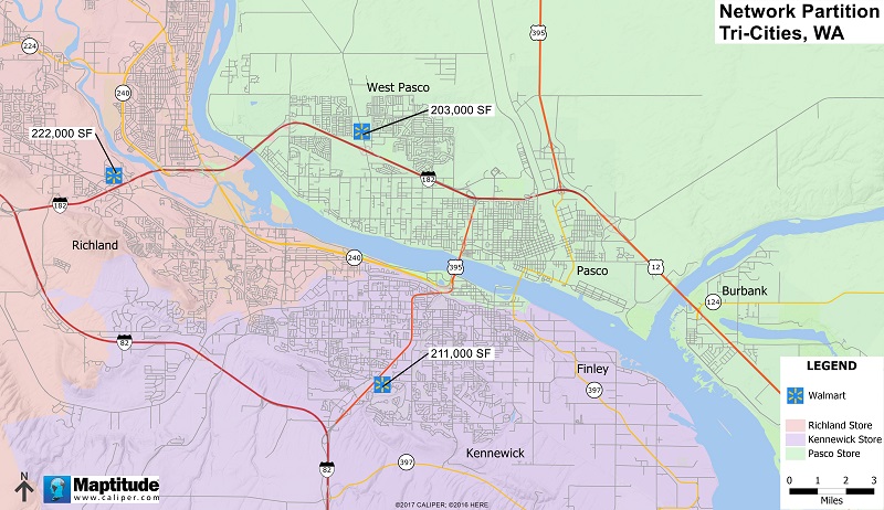
Figure 5. Network Partitioned Bands.
As illustrated, the primary weakness of this method is when the Network Partition band extends across a physical barrier, the physical barrier will generally nudge people to the location on their side of the physical barrier.
5.6 Reilly's "Law" of Retail Gravitation and the Huff Model
Gravity modeling provides an additional method for examining competition and potential shopping patterns around a retail location (Kures, 2011). Other trade area approximation methods discussed do not offer any prediction capabilities. The gravity model attempts to predict the likelihood that a customer will shop at a given location based on distance and the attraction that location offers (Kures, 2011). The model can account for the distribution and attractiveness of competing locations, along with distance the customer will need to travel (Church, 2008).
An early attempt at predicting shopping potential was in 1931 by William J. Reilly. According to Reilly's "law," customers are willing to travel longer distances to larger retail centers given the higher attraction they present to the customer (Reilly 1931). Based on Reilly's formulation, the attractiveness of a center becomes the size (mass) within the physical law of gravity (Reilly 1931).
Equation 1.

Like most other modeling, Reilly’s “law” assumes the geographic study area is flat and there are no physical barriers, to modify a customer's decision of where to travel to buy goods (Church, 2008). Alternatively, Reilly’s “law” also assumes customers are otherwise indifferent to surroundings, including socioeconomic issues such as crime, safety or sales tax rates, as these are not taken into account (Church, 2008).
In 1963, David Huff took Reilly's "law," to the next level, and added a probabilistic feature to the model (Huff, 1964). The Huff Model has been applied in predicting customer spatial behavior. The probability (Pij) that a customer located at i will choose to shop at store j is calculated according to the following equation (Huff 1964).
Equation 2.

As shown, the equation calculates the probability of a person living in one area and may shop in another area, as well as the ability to attract customers from surrounding areas. The α parameter is an exponent to which a store’s attractiveness value is raised, to account for nonlinear behavior of the attractiveness variable (Esri, 2008). The β parameter models the rate of decay in the drawing power as potential customers are located further away from the store (Esri, 2008). An increasing exponent would decrease the relative influence of a store on more distant customers.
When using the Huff Model, the trade area is expressed as a continuous line of probabilities for each location in the analysis (Church, 2008). The point of indifference becomes the point of equal probability that a customer will visit one location or another (Huff, 1964). The advantage of the Huff's Model is that it leaves room for customer choice.
Figure 6 illustrates the model without a parameter estimation or customer spotting data. A typical value for an attractiveness parameter α is 1, and for the distance decay parameter β value of 2. With the default values, this method is generally better than other methods based on the spatial monopoly concept (Jones, 1990).

Figure 6. Huff Model probability analysis using store square footage as a measure of attraction.
As illustrated, store square footage was used as an attractiveness variable, which can be easily determined. A customer probability surface grid size will vary depending on the geographic extent and interpolation efficiently. A potential customer is assumed to be located within every grid cell, so an even distribution of population. The probability of a customer patronizing a selected location is positively related (directly proportional) to the attractiveness of location (store size) and negatively related (inversely proportional) to the distance between the location and the customer, given the presence of competing locations (Huff, 1963). The Huff Model does not take of physical barriers or the road network into consideration.
References
- Applebaum, W. (1966). Methods of determining store trade areas, market penetration, and potential sales. Journal of Marketing Research 3(2), 127-141.
- Birkin, M., Clarke, G., and Clarke, M. (2002). Retail Geography and Intelligent Network Planning. Wiley: New York.
- Church R. L. and Murray, A. T. (2009). Business Site Selection, Location Analysis, and GIS. Hoboken, NJ: John Wiley & Sons.
- Ghosh, A. and McLafferty, S. (1987). Location Strategies for Retail and Service Firms. Lexington Books: Lexington, MA
- Huff, D. L. (1963). A Probabilistic Analysis of Shopping Center Trade Areas. Land Economics, 39(1), 81-90.
- Huff, D. L. (1964). Defining and Estimating a Trading Area. The Journal of Marketing, 28(3), 34-38.
- Jones, K. and Simmons, J. (1990). The Retail Environment, Routledge: London.
- Kures, M. and Ryan, B. (2011). Downtown and Business District Market Analysis. University of Wisconsin Extension, Madison, WI.
- Myles, A. (2003). Understanding Your Trade Area: Implications for Retail Analysis. Mississippi State University Extension: Starkville, MS.
- Pick, J., Greene, R. P., and Stager, J. C. (2005). Geographic Information Systems in Business. IGI Global.
- Reilly, W. J. (1931). The Law of Retail Gravitation. Knickerbocker Press.
- Rice, M.D., and Hernandez, T. (2016). Perspectives on an evolving field: Location intelligence as represented at the first 35 years of the Applied Geography Conference. Papers in Applied Geography 2(3), 271-283.
- Shields, M. and Kures, M. (2007). Black out of the blue light: An analysis of Kmart store closing decisions. Journal of Retailing and Consumer Services 14, 259-268.
- Thrall, G. (2002) Business Geography and New Real Estate Market Analysis. New York: Oxford University Press.
- Xu, Y., & Liu, L. (2004). GIS based analysis of store closure: a case study of an Office Depot Store in Cincinnati. In Proceedings of 12th Int. Conf. on Geoinformatics (pp. 533-540).
Learning outcomes
-
58 - Classify the different metrics that can be used to measure or quantify “attractiveness” for a retailer.
Classify the different metrics that can be used to measure or quantify “attractiveness” for a retailer.
-
69 - Compare and contrast data-driven rings differ with simple rings accounting for their suitability in different settings.
Compare and contrast data-driven rings differ with simple rings accounting for their suitability in different settings.
-
497 - Describe the appropriate context for using simple rings, and identify the limitations and how issues like population density or income changes be accounted for.
Describe the appropriate context for using simple rings, and identify the limitations and how issues like population density or income changes be accounted for.
-
743 - Differentiate between drive-time rings and network partitions, including their utility for retail settings. .
Differentiate between drive-time rings and network partitions, including their utility for retail settings. .
-
821 - Discuss the concept of Census geographies, demography, and the origins of market segmentation, and the role that plays in retail GIS.
Discuss the concept of Census geographies, demography, and the origins of market segmentation, and the role that plays in retail GIS.
-
836 - Discuss the factors which influence site selection, such as available land or AADT's (Annual Average Daily Trips).
Discuss the factors which influence site selection, such as available land or AADT's (Annual Average Daily Trips).
-
963 - Examine how location relates to customer behavior, and how this might differ in an urban versus a suburban or rural setting.
Examine how location relates to customer behavior, and how this might differ in an urban versus a suburban or rural setting.
-
1020 - Explain how Drive-Time Rings account for physical barriers and the relative importance of road speeds.
Explain how Drive-Time Rings account for physical barriers and the relative importance of road speeds.
-
1075 - Explain how Thiessen Polygons account for physical barriers and how they can be used in retail settings.
Explain how Thiessen Polygons account for physical barriers and how they can be used in retail settings.
-
1280 - Identify additional tools that can be incorporated along with the Huff Model to get a more accurate trader area and/or to take into consideration of physical travel barriers.
Identify additional tools that can be incorporated along with the Huff Model to get a more accurate trader area and/or to take into consideration of physical travel barriers.
-
1287 - Identify and describe the limitations of drive-time rings in different settings and how GIS manages these.
Identify and describe the limitations of drive-time rings in different settings and how GIS manages these.
-
1311 - Identify data sources that can be integrated into network partition models.
Identify data sources that can be integrated into network partition models.
-
1341 - Identify sources of data used for analysis within retail GIS and describe how the data are integrated.
Identify sources of data used for analysis within retail GIS and describe how the data are integrated.
-
1550 - Retail sales are a function of market characteristics (Jones, 1990), and important characteristics include customers' income, location, demographics and lifestyle (the latter two are often combined into the term "psychographics"). Explain the role of ea
Retail sales are a function of market characteristics (Jones, 1990), and important characteristics include customers' income, location, demographics and lifestyle (the latter two are often combined into the term "psychographics"). Explain the role of each of these characteristics plays when a retailer considers a location.
-
1555 - Review the limitations of the Huff model in its pure form.
Review the limitations of the Huff model in its pure form.
Related topics
Additional resources
- Buckner, R.W. (1998) Site Selection: New Advancement in Methods and Technology. Chain Store Publishing Corp: New York, NY
- Caliper (2017) Maptitude Mapping Software. Caliper Corporation: Newton, MA. http://www.caliper.com/maptovu.htm
- Caliper (2017) Maptitude Mapping Software Brochure. Caliper Corporation: Newton, MA. http://www.caliper.com/pdfs/maptitude-mapping-software-brochure.pdf
- Esri (2003) Parameter Estimation in the Huff Model. Esri: Redlands, CA. https://www.esri.com/news/arcuser/1003/files/huff.pdf
- Esri (2008) Calibrating the Huff Model Using ArcGIS Business Analyst. Esri: Redlands, CA. https://www.esri.com/library/whitepapers/pdfs/calibrating-huff-model.pdf
- Esri (2015) Business Analyst Online Brochure. Esri: Redlands, CA. http://www.esri.com/library/fliers/pdfs/bao.pdf
- Esri (2017) Tapestry Segmentation. Esri: Redlands, CA. http://www.esri.com/data/tapestry
- Pitney Bowes (2008) MapInfo Professional. Pitney Bowes: Troy, NY. https://www.pitneybowes.com/us
- Rice, M.D. (2017) GEOG 4220/5220: Applied Retail Geography http://www.murrayrice.com/geog-4220.html