Open map List

[DM-02-011] Hierarchical Data Models

As the geographic reality naturally follows hierarchical structures, the hierarchical data models have been widely adopted in multiple approaches of geospatial information science and systems. These approaches include (a) a rigorous conceptual representation of real-world features to explain the human perception of the geographic space; (b) a series of indexing mechanisms for both raster and vector datasets to either accelerate their algorithmic processing, such as their retrieval from big data repositories, or compress their volume and storage requirements; (c) the modelling and retrieval of geospatial content to implement efficient mapping services over the web; and (d) the development of advanced geospatial reference frameworks to effectively support a seamless integration of heterogeneous and multi-resolution geospatial data for the whole planet. This article provides an overview of how hierarchical data models can support these areas through a series of illustrated examples. Specifically, the article explains the principles of the Tomlin’s conceptual representation model, the index structures of quadtrees and R-trees, the tile maps and related conventions of online map providers, and the discrete global grid systems as a partitioning approach to divide the Earth’s surface into a group of uniform cells at various levels of resolutions.

Author and citation

Stefanakis, E. (2023). Hierarchical Data Models. The Geographic Information Science & Technology Body of Knowledge (4th Quarter 2023 Edition). John P. Wilson (Ed.). DOI: https://doi.org/10.22224/gistbok/2023.4.3.

Explanation

Introduction
Conceptual Representation of Reality
Index Structures for Raster and Vector Data
Indexing of Tile Maps
Discrete Global Grid Systems

1. Introduction

A hierarchical data model is a model that organizes the data into a tree-like structure where data entries are connected through one-to-many or parent-child links (a.k.a. relationships). As many geographic features naturally follow a hierarchical structure, hierarchical data models have been widely adopted in geography and geosciences. For example, the Earth contains continents, which contain continental sections, which contain countries, which contain regions, which contain cities, which contain districts, which contain buildings, which contain houses, which contain rooms, which contain furniture, etc.

The hierarchical data models have been widely adopted since the early stages of geospatial data processing to facilitate both the representation of the geographic reality and computation of geospatial algorithms in a computer environment. This article provides an overview of how hierarchical data models have been used for (a) the conceptual representation of real-world features; (b) spatial indexing of raster and vector data; (c) indexing of tile maps in geospatial web services; and (d) establishing a multi-resolution framework for global geospatial analysis.

2. Conceptual Representations of Reality

The representation of reality in a computer involves two models (Figure 1): (i) representation model of reality, and (ii) data model. The representation model is a conceptual model that leads to the picture of reality as a human perceives that reality. The data model implements a human’s perception in a computer environment.

Figure 1. Models for the representation of reality in human’s perception and a computer environment. Source: author.

The representation models of space in a static space address two questions: (a) what is it? and (b) where is it located? The two most common approaches to model the reality and answer these questions are (Figure 2): (a) the perception of space as a collection of discrete entities and (b) the perception of space as a continuous field.

Figure 2. The two basic approaches to represent the reality in a human’s perception. Fig 2a (left) is the perseption of space as a collection of discrete entities and Fig 2b (right) as the perception of space as a continuous field. Source: author.

A representation model, introduced by Tomlin (1992), handles in an elegant manner both perceptions of geographic space. In this general representation model, geographic information can be viewed as a hierarchy of data (Figure 3). At the highest level, there is a map which is a collection of thematic layers (more commonly referred to as layers), all of which are in registration (i.e., they have a common coordinate system) (Figure 4a). Each layer is partitioned into zones (regions), where a zone is a set of individual locations with the same attribute value (Figure 4b).

Figure 3. Tomlin's hierarchical representation model. Source: author.

Figure 4. Tomlin’s model: (a, left) the map layers, and (b, right) the zones on a single layer. Source: author.

Examples of layers are the land-use layer, which is divided into land-use zones (e.g., wetland, river, urban, desert, city, park and agricultural zones), and the road network layer, which contains the roads that intersect the portion of space that is covered by the layer.

Tomlin’s model is very effective as it applies regardless of the approach adopted for the representation of reality (Figure 2). Specifically, this is accomplished by introducing the concepts of zone and location in the hierarchy (Figure 3). Thus, each discrete entity, e.g., a road or a parcel, can be represented as a zone in this model. The zone is defined as the set of locations that make up the road or parcel. On the other hand, a continuous field, e.g., field of vegetation, is represented in the model as a thematic layer, which comprises all locations in space. Tomlin’s model is supplemented by an algebra (a.k.a. map algebra) with which analytical tools, operators, and functions can be applied to perform spatial analysis.

3. Index Structures for Raster and Vector Data

3.1 Quadtree Index Structure

Originally designed for representing, compressing, and analyzing raster geospatial data, such as satellite images and raster GIS layers (Figure 5), the quadtree structure has evolved to also represent vector data as well as indexing map tiles for online map providers. The hierarchical structure of quadtrees has proven very effective in performing certain functions of spatial analysis, such as finding the nearest neighbor, or solving the point-in-polygon problem.

Figure 5. Example of a raster representation (b) for a simplified area with four polygonal features (a). The values assigned to the cells correspond to the first letter of each feature. Source: author.

The quadtree is a hierarchical index structure (Samet, 1990), which organizes the space by recursively dividing it into four regions (a.k.a. quadrants), labelled as {0,1,2,3}. The recursive splitting stops when either the area of a quadrant has met a condition (e.g., it has a unique attribute value for a theme) or the tree has reached its maximum height. The root of the tree corresponds to the entire region. The leaves of the tree are assigned a value for the thematic attribute, which describes the whole or most area of the corresponding region (Figure 6). Figure 7 shows the recursive partitioning of space and the corresponding quadtree for a simplified geographic area with four features (Figure 5).

Figure 6. Example quadtree representation of a simplified square area. Source: author.

Figure 7. Quadtree representation of the study area in Figure 5. The values (letters) assigned to the leaf nodes correspond to the four features of the study area. Source: author.

A variant of the quadtree that can be used to structure vector data (points, lines, and polygons) has the following properties. The space is recursively divided into four regions (quadrants) of the same size. Each vector object is assigned to the smallest quadrant of the tree that entirely contains the object. Therefore, vector objects can be assigned to both non-leaf and leaf nodes of the quadtree. As for the point objects, the partition continues until the maximum allowable height for the tree (or minimum size quadrant) is reached.

Figure 8b (right) shows a quadtree index for the vector data in Figure 8a (left). It is obvious that each node of the tree can be assigned more than one object. The region search algorithm works as follows. For the shaded area Q, the tree is traversed starting from the root and following the paths to descendant quadrants, overlapped partially or fully by Q. If the quadrant is fully covered by the region Q, all entries assigned to the corresponding tree node and all its descendent nodes are reported. If the quadrant is partially covered by the region Q, the objects assigned to the corresponding node are checked for a geometric intersection against Q and are reported if the intersection occurs. The traversal recursively continues at lower levels of the tree through all the nodes whose quadrants intersect the region Q.

Figure 8. A vector quadtree (Fig. 8b, left) and the region search over the vector area Q (Fig. 8a, left). The arrows point to the visited nodes, while all vector objects intersecting the area Q are ticked. Source: author.

3.2 R-tree index structure

The R-tree structure and its variants (R+, R*trees, etc.) are the most efficient hierarchical index structures for vector data adopted by most commercial and open-source database systems, geographic information systems (GIS), and computer aided design (CAD) software.

The principle of the R-tree structure (Guttman, 1984) can be summarized as follows: (a) geometric objects are represented in the index with their minimum bounding rectangle (MBR); (b) these MBRs are recursively grouped into larger MBRs, which are called pseudo-MBRs; and (c) these pseudo-MBRs along with the object MBRs form hierarchies by being structured in a tree index. Figure 9 shows the representation of the three types of geometric objects (point, line, polygon) with the corresponding MBRs.

Figure 9. Representation of 2D geometric objects with minimum bounding rectangles (MBRs). Source: author.

Figure 10 presents the MBRs of the objects illustrated in Figure 8a.

Figure 10. Representation of 2D geometries as previously represented in Fig 8a, along with their MBRs. Source: author.

Figure 11 shows the grouping of neighboring MBRs into larger pseudo-MBRs, which are further organized into an R-tree structure.

Figure 11. MBR grouping (Fig 11a, left) and organization in an R-tree (Figure 11b, right). Example region search over the area Q. The arrows point to all visited nodes, while all MBRs of vector objects intersecting the area Q are ticked. Source: author.

The R-tree is a balanced tree, i.e., all leaf-nodes lie at the same level. The actual objects are indexed at the leaf nodes of the tree, which accommodate their MBRs. Each node of the tree has a number of children, which varies between a maximum value (M) and a minimum value (m), in accordance with the B+tree structure for alphanumeric data (Sedgewick and Wayne, 2011). The height of the tree for indexing N objects is less than or equal to logm(N-1), which guarantees high performance search results.

The region search algorithm works as follows. For a search region Q (Figure 11a), the tree is traversed starting from the root. At each node, the intersection of its pseudo-MBR against the region Q is checked. If they intersect, the traversal continues recursively to the node’s descendants. When a leaf node is reached, all the MBRs indexed by the node intersecting Q are reported in the query result.

4. Indexing of Tile Maps

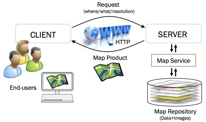
To meet the high demand of rendering and delivering complex and high quality basemaps over the web (Figure 12), online map providers, like Google Maps, OpenStreetMap, and ArcGIS Online, pre-compute and cache image files, a.k.a. tile maps of the globe at various resolutions, themes, and languages (Figure 13) (Stefanakis, 2017). The creation of tile maps depends on a series of parameters, such as the shape and size of tiles (images), zoom levels, subdivision scheme of a tile to produce tiles at a higher resolution, encoding of map tiles, map projection, map content, etc.

Figure 12. Abstract framework of interaction between online map service providers (server) and end-users (client) over the web. Source: author.

Figure 13. Various types of map products requested by end users: (a, left) multi-location mapping; (b, center) multi-resolution representation; and (c, right) multi-theme and multi-language mapping. Source: author.

Google Maps conventions, also adopted by the major online map providers, for these parameters are as follows. All tile maps are square-shaped and equal sized images of 256x256 pixels, forming a hierarchy like a quadtree structure. The world is rendered on a single tile (the root of the tree) at the outer most zoom level 0. This layout depicts the earth as an absolute square that excludes the polar areas in the Web Mercator projection on the WGS’84 datum. Each tile (tree node) at any zoom level k is subdivided into 4 disjoint square equal-sized 256x256 pixel tiles at the subsequent zoom level k+1. The number of tiles at zoom level k is equal to 4^k, e.g., at zoom levels 3 and 17, there are 64 and 17,179,869,184 tiles, while the ground resolution is approx. 20km and 120cm per pixel, respectively (Figure 14). The encoding of a tile at zoom level k is described by a pair of integers (x,y), where x is the column number of the tile, starting from the longitude of 180 degrees and heading East, and y is the row number of the tile, starting from the latitude of approx. 85 degrees North and heading South (Figure 15).

Figure 14. Google Maps’ hierarchical model of tiles. Source: author.

Figure 15. Google Maps’ tiling scheme. The first three zoom levels, the tiles, and their encoding. All tiles are square-shaped of 256x256 pixels. Source: author.

5. Discrete Global Grid Systems

Discrete Global Grid System (DGGS) is a partitioning approach to divide the Earth’s surface into a group of uniform cells at various levels of resolutions. DGGS offers an alternative hierarchical geospatial reference framework with increasing popularity over the last few years (Gibbs 2021) as it can effectively support the sampling, storage, modeling, processing, analysis, integration, and visualization of voluminous and heterogeneous geospatial data.

A common way to construct a DGGS includes the following three steps:

Discretization of the Earth Surface into planar cells using a platonic solid.
Refinement of the initial cells to a target resolution level.
Projection of the Earth’s surface to the refined planar cells using an equal-area projection method.

A platonic solid is a convex polyhedron that consists of polygonal faces with the same number of faces meeting at each vertex. In addition, these faces are congruent (identical in shape and size) and regular (all angles are equal and all sides equal). Five solids meet these criteria and are named based on the number of their faces (Figure 16): Tetrahedron (four faces), Cube (six faces), Octahedron (eight faces), Dodecahedron (twelve faces), and Icosahedron (twenty faces). The initial cells of a platonic solid can be refined to any resolution following a recursive subdivision.

Figure 16. Platonic solids. From left to right: Tetrahedron, Cube, Octahedron, Dodecahedron, and Icosahedron. Source: author.

A DGGS based on the octahedron (Goodchild and Shiren, 1992) creates a hierarchical structure of spherical triangles for the entire globe with cells of similar size and shape at variable resolutions, depending on the application requirements and the desired level of detail. According to this structure, the globe is divided initially (first level of segmentation) into eight disjoint spherical triangles. Four of these located on the northern hemisphere of the earth and the remaining four on the southern hemisphere. All the triangles of the northern hemisphere share the North Pole as a common vertex. The other two vertices of these triangles lie on the equator and by triangle in the following pairs of geographic longitudes: 0° and 90°, 90° and 180°, 180° and 270°, 270° and 0°, respectively. In a similar way, the four triangles of the southern hemisphere are defined. Figure 17a highlights one of the eight initial triangles. Then, each of the eight triangles is further divided (second level segmentation) into four new spherical triangles. The new triangles are defined by connecting the medoids of the adjacent edges in the original triangle with spherical edges to produce equal-sized triangles. Figure 17b schematically shows the second level segmentation of one of the eight spherical triangles. The segmentation recursively continues to new triangles until the desired level of resolution is reached (Figure 17c).

Figure 17. Schematic representation of the recursive partition of a spherical triangle. Source: author.

Figure 18 shows an example DGGS based on the icosahedron, the most adopted platonic solid for DGGS, using a hexagonal grid (Sahr, et al., 2003). The first level of refinement includes the truncation (cut off) of the 12 icosahedron vertices. This truncation creates 12 new pentagon faces and leaves the original 20 triangle faces as regular hexagons, while the length of the edges is one third of that of the original icosahedron edges. The truncated icosahedron is the model for the traditional soccer ball.

The faces of the truncated icosahedron can be recursively subdivided to reach the target resolution. Figure 19 shows an example subdivision of the truncated icosahedron hexagonal faces at the next two resolution levels, based on the hexagonal grid. Figure 20 shows the result of the subdivision of a spherical surface using the initial icosahedron and a finer resolution level using the hexagonal grid. Finally, Figure 21 shows the representation of a coastal area at two different resolution levels on a hexagonal DGGS.

References

- Gibb, R. (Ed.) (2021). Topic 21 - Discrete Global Grid Systems - Part 1 Core Reference system and Operations and Equal Area Earth Reference System. Open Geospatial Consortium.
- Goodchild, M. F. and Shiren, Y. (1992). A hierarchical spatial data structure for global geographic information systems. CVGIP: Graphical Models and Image Processing, 54(1):31-44.
- Guttman, A. (1984). R-trees: A dynamic index structure for spatial searching. In Proceedings of the 1984 ACM SIGMOD International Conference on Management of Data, 14(2):47-57.
- Sahr, K., White, D., and Kimerling, A.J. (2003). Geodesic Discrete Global Grid Systems. Cartography and Geographic Information Science, 30(2):121-134.
- Samet, H. (1990). The Design and Analysis of Spatial Data Structures. Addison Wesley Publishing Company, Inc.
- Sedgewick, R., and Wayne, K. (2011). Algorithms. 4th Edition. Addison-Wesley Professional Publishers.
- Stefanakis, E. (2017). Web Mercator and Raster Tile Maps: Two Cornerstones of Online Map Service Providers. Geomatica Journal, 71(2):100-109.
- Tomlin, C. D. (1990). Geographic Information Systems and Cartographic Modeling,1st Edition. Englewood Cliffs, New Jersey: Prentice-Hall (now Pearson Education).
Learning outcomes
-
1682 - Explain the importance of hierarchical data models in geospatial information systems
Explain the importance of hierarchical data models in geospatial information systems
1683 - Describe Tomlin's conceptual model of reality.
Describe Tomlin's conceptual model of reality.
1684 - Explain how quadtrees and R-trees index raster and vector datasets.
Explain how quadtrees and R-trees index raster and vector datasets.
1685 - Describe the indexing scheme for online tile maps.
Describe the indexing scheme for online tile maps.
1686 - Explain the hierarchical model of discrete global grid systems for multi-resolution representation of geospatial data.
Explain the hierarchical model of discrete global grid systems for multi-resolution representation of geospatial data.