[DM-03-066] Spatial Indexing

Zhang, X and Du, Z. (2017). Spatial Indexing. The Geographic Information Science & Technology Body of Knowledge (4th Quarter 2017 Edition), John P. Wilson (ed). DOI: 10.22224/gistbok/2017.4.12

1. Overview
2. Spatial Index in Different Databases
3. Space-driven Structures
4. Data-driven Structures
5. Discussion

1. Overview

Spatial Index is a data structure that allows for accessing a spatial object efficiently. It is a common technique used by spatial databases. A variety of spatial operations needs the support from spatial index for efficient processing:

Range query: Finding objects containing a given point (point query) or overlapping with an area of interest (window query).

Spatial join: Finding pairs of objects that interact spatially with each other. Intersection, adjacency, and containment are common examples of spatial predicates to perform spatial joins.

K-Nearest Neighbor (KNN): Finding the nearest K spatial objects in a defined neighborhood of a target object.

Here is a simple test executing the SELECT statement with and without a spatial index, finding corresponding features from three different datasets by a given point. Both SELECT operations yield the same results, however, the execution time increases when the data volume gets larger. Without indexing, any search for a feature would require a "sequential scan" of every record in the database, resulting in a much longer processing time.

Figure 1. The point query test in Mysql 5.17.19 using 2017 TIGER national geodatasets. Time is measured in milliseconds, which is the precision of Mysql. 

In order to reduce the cost of calculating the complex shape of spatial object during the search traversal, we use approximations of the complex object geometries. The most commonly used approximation is the minimum bounding rectangle, or MBR, which is also called minimum bounding box, or MBB. An MBR is a single rectangle that minimally encloses the geometry in 2D plane, as shown in Figure 2(a). It can also be extended to higher dimensions, such as a 3D MBR as in Figure 2(b).

Figure 2. Minimum bounding rectangles of 2D objects (a) and 3D objects (b). 

In a 2D plane, an MBR is defined by four coordinates, (xmin ymin) and (xmaxymax). These coordinates represent the following:

• xmin is the x-coordinate of the lower-left corner of the bounding box.
• ymin is the y-coordinate of the lower-left corner of the bounding box.
• xmax is the x-coordinate of the upper-right corner of the bounding box.
• ymax is the y-coordinate of the upper-right corner of the bounding box.

When performing a spatial operation on a collection of indexed spatial objects, we first use MBR instead of the shape of spatial object to test the relation. By filtering spatial objects outside the MBR, time consuming on spatial predicates will reduce significantly. Then, in a second step, we use the actual shape in the subset of first step to test the spatial relation with target object.

2. Spatial Index in Different Databases

Different data sources use different data structures and access methods. Here we list two well-known spatial indices as well as databases which use them. The categorization system proposed by Riguax et al. (2002) is employed here for illustration:

Space-driven structures. These data structures are based on partitioning of the embedding 2D space into cells (or grids), mapping MBRs to the cells according to some spatial relationship (overlap or intersect). Commercial databases like IBM DB2 and Microsoft SQL Server use these methods. Besides, Esri also implement its spatial data access method on geodatabases using space-driven structures.

Data-driven structures. These data structures are directly organized by partition of the collection of spatial objects. Data Objects are grouped using MBRs adapting to their distribution in the embedding space. Commercial databases like Oracle and Informix as well as some open-source databases, PostGIS and MySQL, use these data structures.

3. Space-driven Structures

Space-driven structures of spatial objects are instinctively using partitioning and mapping strategies to decompose 2D plane into a list of cells, and can be used in spatial extensions with B+-tree, which is dynamic and efficient in memory space and query time. Although some of the indices can handle with arbitrary dimensions, we here describe four common partitioning structures in 2D case.

3.1 Fixed grid index

Fixed grid index is an n×n array of equal-size cells. Each one is associated with a list of spatial objects which intersect or overlap with the cell. Figure 3 depicts a fixed 4×4 gird indexing a collection of three spatial objects.

Figure 3. An example of a fixed grid structure.

To further decrease the redundancy, a hierarchical uniform decomposition of the plane can be enabled. The index-creation process decomposes the plane into an m-level grid hierarchy (Microsoft SQL Server uses 4 level and IBM DB2 uses 3 level). These levels are referred to as level 1 (the top level), level 2, level 3… level m. The decomposition is more complex when the level gets higher. As shown in Figure 4, each cell at a higher level is decomposed into a 4x4 grid at the next level.

Figure 4. A four-level fixed grid structure.

These grid hierarchy cells are numbered in a linear fashion called space-filling curves. They are useful because it partially preserves proximity, that is, two cells close in 2D plane are likely to be close in the sequential order. There are different spatial filling curves and here we use the z-order curve Figure 5(a) as an example of spatial filling curves. The Hilbert curve in Figure 5(b) is also well known.

Z-order labels each cell like a complete quadtree and numbers each quadrant in binary format 00, 01, 10, 11. The number for a node is the concatenation of the quadrant numbers for each of its ancestors, starting at the root. For example, in Figure 5(a), "0" denotes a binary 00 for the top left, "1" denotes a binary 10 for the top right, and so forth. And the 2D plane gets further filling at a depth of 1, 2 and 3. This order is also called Morton code, which is used in raster storage.

Figure 5. Two common space filing curves: z-order (a) and Hilbert curve (b)

3.2 Quadtree

Quadtree is a very popular spatial indexing technique. It is a specialized form of grid in which the resolution of the grid is varied according to the density of the spatial objects to be fitted.

In a Quadtree, each node represents a bounding box covering some part of the space being indexed, with the root node covering the entire area. Each node is either a leaf node which contains one or more indexed points, and no children, or it is an internal node, which has exactly four children, one for each quadrant obtained by dividing the area covered in half along both axes. This is also how the name “quadtree” comes from.

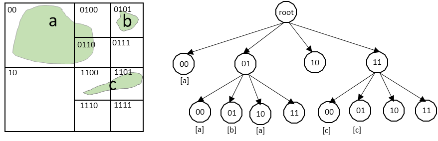
Figure 6. A representation of a quadtree structure. 

3.3 KD-tree

The general idea behind KD-tree is that it is a binary tree, each of its nodes represents an axis-aligned hyper-rectangle as Figure 7 shows. Each node specifies an axis and splits the set of points based on whether their coordinate along that axis is greater than or less than a particular value (Rigaux, 2012; Maneewongvatana, 1999), such as the coordinate median.

Figure 7. A representation of a KD-tree structure. 

The KD-tree can be used to index a set of k-dimensional points. Every non-leaf node divides the space into two parts by a hyper-plane in the specific dimension. Points in the left half-space are represented by the left subtree of that node and points falling to the right half-space are represented by the right subtree.

The hyper-plane formation is in the following way. First, choose one dimension as split axis and a middle point, such as “x” axis and point “f” in Figure 7. Then every point finds its position in the tree depending on its relative value to the middle point. All points in the subtree with a smaller "x" value than the point “f” will appear in the left subtree and all points with larger "x" values will be in the right subtree. Continue to split axes and repeat the above steps to construct a KD-tree.

3.3 Geohash

Gustavo Niemeyer invented Geohash in 2008 with the purpose of geocoding specific points as a short string to be used in web URLs. He entered the system into the public domain by publishing a Wikipedia page on February 26, 2008 (Fox et al., 2013; Geohash, 2017).

A Geohash is a binary string in which each character indicates alternating divisions of the global longitude-latitude rectangle. The process of partitioning spatial plane can be seen from Figure 8. The first division splits the rectangle into two squares with a Geohash code of "0" and "1." Spatial objects locates at the left of the vertical division have a Geohash beginning with ‘0’ and the ones in the right half have a Geohash beginning with "1" as its first prefix. Then, data at each side is further split horizontally: objects that are above the line receive "0" and the ones below receive "1" as their second prefix. The patterns continues to split until the desired resolution is reached. Every Geohash rectangle can be decomposed into four sub-hashes that are visited in a self-similar z-order curve.

In order to make Geohash more useful for the web, the inventor assigned a plain text, base-32 and base-36 encoding for his web service to get a short web URL. The length of Geohash could range from 1 (in Figure 8) to 12. A longer Geohash has a finer precision.

Figure 8. An example of a Geohash (with a hash code "v")

4. Data-driven Structures

The difference between space-driven structures and data-driven structures is that the latter use the idea of a spatial containment relationship instead of the order of the index. These structures adapt themselves to the MBR of the spatial objects and they are part of the R-tree family.

4.1 R-tree

For a layer of geometries, an R-tree index consists of a hierarchical index on the MBRs of the geometries in the layer (Guttman, 1984). This hierarchical structure is based on the heuristic optimization of the area of MBRs in each node in order to improve the access efficiency.

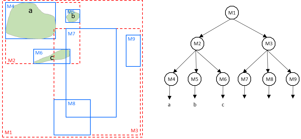
Figure 9. R-Tree Hierarchical Index in Minimum Bounding Rectangles (MBRs)

In Figure 9, M4 through M9 are MBRs of spatial objects in a layer. They are the leaf nodes of the R-tree index, and contain minimum bounding rectangles of spatial objects, along with pointers to the spatial objects. M2 and M3 are parents of the leaf nodes. M1 is the root, containing all the MBRs. This R-tree has a depth of three.

This kind of containment relationship could be extended to higher dimensions and has a similar construction and query methods. Unlike the space-driven structures, spatial objects here only belong to one of the tree leaves and MBRs have overlap between nodes, such as M7 and M8 in Figure 9.

4.2 Variants of R-Tree

Variants of the R-tree provide several improvements to the construction process (Beckmann et al., 1990), especially with regards to inserting and splitting of nodes. Essentially, these improvements aim at optimizing the following parameters: node overlapping, area covered by a node, and perimeter of a node’s directory rectangle. The perimeter of a node’s directory rectangle is representative of the shape of the MBR because, given a fixed area, the shape that minimizes the MBR perimeter is the square (in 2D) or cube (in 3D). There are no well-founded techniques to simultaneously optimize these three parameters. Thus, different variants bring different improvements with respect to the original R-tree. Three of the variants are described below.

• The R∗-tree approach assumes the split to be performed along one axis (say, x-axis), and explores all possible distributions of objects above or below the split line. Another characteristic is that R*-tree forces one to reinsert the same objects when structures are updated. This alleviates some degraded conditions.
• R-tree Packing is also a well-known type of data structure. In this case, we use a pre-processing phase that sorts MBRs according to their location (for example, the x coordinate of the centroid) and then construct the nodes in a way that involves less overlap.
• In the R+-tree, the MBR of nodes at a given level do not overlap. Objects that cross different MBRs appear twice or more. This is similar to some space-driven structures. As a result, a single path is followed from the root to a leaf for a point query.

5. Discussion

5.1 Performance measurements

To compare different spatial indices and evaluate the efficiency of an improved spatial index, the following performance factors can be analyzed (Bentley & Friedman, 1979):

• Preprocessing Cost. The cost of preprocessing spatial objects in multi-dimension space into a data structure;
• Storage Cost. The storage required by the data structure; It is idea when the space is fully used and not biased;
• Query Cost. The search time or query cost, as was measured in Figure 1.

These cost factors can be analyzed in terms of their average or worst case. Besides, we should take "dynamicity" into consideration as well, because in many applications one may desire to execute various utility operations on data structures, such as insertion and deletion.

5.2 Efficiency degrade

A substantial number of insert and delete operations may result in efficiency degradation, which may adversely affect query performance.

In the grid index case, if the MBR contains or intersects with several grid cells such as object ‘a’ in Figure 3, it will be assigned to several neighbor cells. When the collection size get closer to the grid size, it will lead to an increase in the index size and therefore causes an efficiency degradation.

The performance of an R-tree index structure for queries is roughly proportional to the area and perimeter of the index nodes of the R-tree. The original ratio of the area at the root (topmost level) to the area at level 0 can change over time based on updates to the table, and there is degradation in that ratio when it increases significantly.

5.3 Evaluation and improvement

A space-driven spatial index has the advantage that the structure of the index can be created first, and data will then be added gradually without requiring any change to the index structure; indeed, if a common grid is used by disparate data collecting and indexing activities, such indices can easily be merged from a variety of sources. On the other hand, data driven structures such as R-trees can be more efficient for data storage and faster in search execution time, but they are generally tied to the internal structure of a given data storage system.

In the meantime, there has been a recent explosion in the amount of spatial data produced by various devices such as smart phones, satellites, and medical devices. Researchers and practitioners worldwide want to take advantage of different technologies to speedup spatial operations of large-scale spatial data. For example, Fox et al. (2013) utilized Geohash within Accumulo, a non-relational distributed data, to complete the spatio-temporal queries on spatial objects. Jensen, Lin, and Ooi (2004) relied on R+-tree to handle queries and update operations on trajectory point data. More researchers have extended Hadoop (Eldawy & Mokbel, 2015), Spark (Du et al. 2017) and Storm (Zhang et al., 2016) to perform spatial file splitting jobs in different spatial operation scenes. Spatial indexing techniques are playing a central role in time-critical applications and the manipulation of spatial big data.

Bertino, E., Ooi, B. C., Sacks-Davis, R., Tan, K. L., Zobel, J., Shidlovsky, B., & Andronico, D. (2012). Indexing techniques for advanced database systems (Vol. 8). Springer Science & Business Media.

Obe, R. O. & Hsu, L. S. (2015). PostGIS in action. Manning Publications Co.

References

- Beckmann, N., Kriegel, H. P., Schneider, R., & Seeger, B. (1990, May). The R*-tree: an efficient and robust access method for points and rectangles. In ACM Sigmod Record (Vol. 19, No. 2, pp. 322-331). ACM.
- Bentley, J. L. & Friedman, J. H. (1979). Data structures for range searching. ACM Computing Surveys (CSUR), 11(4), 397-409.
- Du, Z., Zhao, X., Ye, X., Zhou, J., Zhang, F., & Liu, R. (2017). An Effective High-Performance Multiway Spatial Join Algorithm with Spark. ISPRS International Journal of Geo-Information, 6(4), 96.
- Eldawy, A., and Mokbel, M. F. (2015). SpatialHadoop: A MapReduce Framework for Spatial Data. In Proceedings of the 2015 IEEE 31st International Conference on Data Engineering, Seoul, Korea (South), 2015, pp. 1352-1363.
- Fox, A., Eichelberger, C., Hughes, J., & Lyon, S. (2013, October). Spatio-temporal indexing in non-relational distributed databases. In Big Data, 2013 IEEE International Conference on (pp. 291-299). IEEE.
- Geohash. (2017, May 10). In Wikipedia, The Free Encyclopedia. Retrieved 21:02, October 22, 2017
- Guttman, A. (1984). R-trees: A dynamic index structure for spatial searching. In Proceedings of the 1984 ACM SIGMOD International Conference on Management of Data, 14(2):47-57.
- Jensen, C. S., Lin, D., & Ooi, B. C. (2004, August). Query and update efficient B+-tree based indexing of moving objects. In Proceedings of the Thirtieth international conference on Very large data bases - Volume 30 (pp. 768-779). VLDB Endowment.
- Kothuri, R. K. V., Ravada, S., & Abugov, D. (2002, June). Quadtree and R-tree indexes in oracle spatial: a comparison using GIS data. In Proceedings of the 2002 ACM SIGMOD International Conference on Management of data (pp. 546-557). ACM.
- Maneewongvatana, S, & Mount, D. M. (1999, December). It's okay to be skinny, if your friends are fat. In Center for Geometric Computing 4th Annual Workshop on Computational Geometry (Vol. 2, pp. 1-8).
- Rigaux, P., Scholl, M. and Voisard, A. (2002). Spatial Databases: With Application to GIS. San Francisco:Morgan-Kaufmann.
- Zhang, F., Zheng, Y., Xu, D., Du, Z., Wang, Y., Liu, R., & Ye, X. (2016). Real-Time Spatial Queries for Moving Objects Using Storm Topology. ISPRS International Journal of Geo-Information, 5(10), 178.
Learning outcomes
-
129 - Compare and discuss the relative performance of different spatial indices.
Compare and discuss the relative performance of different spatial indices.
292 - Define the concept of a spatial index and what kind of spatial operations it is related to.
Define the concept of a spatial index and what kind of spatial operations it is related to.
326 - Demonstrate how different data structures works for spatial queries and spatial join.
Demonstrate how different data structures works for spatial queries and spatial join.
501 - Describe the basic category of spatial index and name some common data structures of spatial databases.
Describe the basic category of spatial index and name some common data structures of spatial databases.
1399 - Implement point query or window query algorithms that retrieve geospatial data using basic index structures
Implement point query or window query algorithms that retrieve geospatial data using basic index structures
1631 - Understand how to build spatial indexes in both commercial and open-source databases and be aware of what the strategies they use.
Understand how to build spatial indexes in both commercial and open-source databases and be aware of what the strategies they use.
Related topics
Additional resources