[DM-01-081] Array Databases

Haynes, D. (2019). Array Databases. The Geographic Information Science & Technology Body of Knowledge (3rd Quarter 2019 Edition), John P. Wilson (ed.). DOI: 10.22224/gistbok/2019.3.2

1. Array Database Overview
2. Array Database Operations
3. Spatial Analysis for Array Databases
4. Future Directions

1. Array Database Overview

Array Databases are a class of databases that store, manage, and analyze data whose natural structures are arrays. Currently, there are a few systems, including SciDB, RasDaMan, MonetDB, and Google Earth Engine that are array databases (Baumann et al., 2018). The first array database, RasDaMan, was developed in 1999 to store the continuously growing datasets generated from scientific discovery and sensor observations that are typically structured as arrays (Widmann & Baumann, 1999). 

Other platforms and databases have been developed to support arrays. Relational databases, such as PostgreSQL with PostGIS, have been supporting the array datatype since 2012. Oracle GeoRaster is a related project and uses a similar model. However, simulating array structures inside a relational database results in a performance cost. The performance cost is related to the size of the array being larger than the size of the page read within a traditional database (Stonebraker, Brown, Poliakov, & Raman, 2011). 

The need to store and manipulate array data has resulted in many databases and platforms extending their initial architectures to support for multidimensional arrays and the operations necessary to query them. However, extending a platform to support a multidimensional array comes at a performance cost and is not the same as an array database whose primary data structure is an array. 

For example, MonetDB extended its column store database architecture to support multidimensional arrays. Also, they developed a secondary language, SciQL to support array operations (Kersten, Zhang, Ivanova, & Nes, 2011). For Hadoop systems there have been extensions like SciHadoop and SciMate that have extended Hadoop to perform operations on arrays, providing drivers for reading multi-dimensional arrays as well as operations for processing arrays in Map-Reduce (Buck et al., 2011; Wang, Jiang, & Agrawal, 2012). Lastly, as Hadoop has moved from disk-based reads to memory reads with Spark, there have been extensions like SciArray and GeoTrellis (Kini & Emanuele, 2014; Wang et al., 2016). The common theme is that all of these platforms have extended their primary platforms and data structures to incorporate multidimensional arrays. The performance of the array and the operators available for processing arrays vary accordingly. Array Databases address this issue by making the array the primary data structure and using partitioning schemas formatted for arrays.

The two most popular open-source array databases for geospatial analysis are RasDaMan and SciDB. RasDaMan, developed by Dr. Peter Bauman, has been developed explicitly for the geospatial community (Baumann, 2016; Baumann, Dehmel, Furtado, Ritsch, & Widmann, 1998). In comparison, SciDB, developed by Dr. Michael Stonebraker, is a general array database that has been applied to genomics, finance and geospatial analysis (Planthaber, Stonebraker, & Frew, 2012; Stonebraker et al., 2011). MonetDB began supporting array stores with SciSQL in 2007 but is no longer a currently active project (Kersten et al., 2011).

While there are operational differences between the systems, their underlying architectures remain similar. All systems employ a column-store approach for structuring and storing array data. Column-store databases differ from traditional (row-based) databases by the way they store and access data. Row-store databases store data in collections of tuples, in which each field/column of a particular record is stored with the entire record (Figure 1A). Column-store databases arrange and store data by columns/fields (Figure 1B). Array-stores systems use a similar approach to column-store systems in that each variable or band, for example, in satellite imagery is stored independently as a column-store stored field.

Figure 1. Row-store vs. Column-store databases

Column-store approaches are preferred to row-store because they improve the reading and writing access for big data by colocation and storing data that is related to similar locations. Array-stores adopt this technique by allowing the arrays to be structured and stored by their dimensions. For example, each pixel in a raster dataset is tied to specific x and y locations. The array database utilizes dimensions as an opportunity to partition the data, thereby co-locating all pixels that have similar coordinates. This approach is similar to geospatial tiling used for storing and compressing raster spatial data. Data partitioning, breaking a large table or array into smaller elements, is known to increase the performance of large database tables (Pavlo, Curino, & Zdonik, 2012).  When the data is partitioned, and the resulting queries are run, the database only accesses a fraction of the entire dataset. With an array database storing geospatial data, data partitioning allows the array-store database to fetch only the tiles that are necessary for any operation. Another benefit of using these techniques is that it reduces the need for building customized indices that are cumbersome and become outdated as the dataset changes (Abadi, Boncz, & Harizopoulos, 2009). 

The last significant architectural advancement introduced in array stores is the integration of shared-nothing architectures that support deployment within a cloud or grid computing environment. A shared-nothing architecture for a database, means that two or more instances of a database are deployed, each on its node with a portion of the data. Shared-nothing means neither memory or data storage is shared (Stonebraker, 1986). Implementation of this architecture allows for the system to be scaled out on 10s to 100s of nodes with each database instance/node containing a fraction of the entire dataset. By coordinating and distributing the dataset across a network of nodes, the system takes advantage of massively parallel processing (MPP) techniques.  

Array Databases are classified as “NoSQL” databases because they store data in a row structure, and they do not use Structured Query Language (SQL). Accordingly, they have implemented one or more query languages to support interaction with the databases. RasDaMan and SciDB have a primary language often called functional language, which contains primitives for creating, transforming, and modifying arrays. The operator or functions written in the primary language are designed to be embarrassingly parallel so that the system can take advantage of its MPP capabilities. RasDaMan and SciDB also support a second higher-level language, which is similar to Structured Query Language (SQL). RasDaMan’s RASQL and SciDB’s Array Query Language are not SQL dialects but contain a subset of specific SQL clauses that can be translated into the underlying functional languages. Providing the SQL-like languages supports broader audiences for each platform.

2. Array Database Operations

Arrays in an Array Database are equivalent to tables in a Relational Database and have specific Data Definition Languages. For RasDaMan arrays can be defined as a collection, which is one or more n-dimensional arrays or as particular array-type, which is an n-dimensional array (Figure 2). To define an array, the user specifies the data type, upper and lower bounds for each dimension, as well as the array name (Figure 2). Defining a collection in RasDaMan allows for a set of arrays to be logically grouped so that when operations are applied to a collection, they are applied to all associated arrays. SciDB’s array definition is similar to the RasDaMan array-type definition in that the parameters needed to create an array are array name, data type, and the upper and lower bounds for all dimensions (Figure 3). A difference between the RasDaMan and SciDB definitions is that SciDB requires that each band or field have a name, whereas with RasDaMan fields are unnamed.

Figure 2. Defining Arrays with RasDaMan, RASQL

Figure 3. Define Array with SciDB, AFL

2.1 Defining an Array 

Both SciDB and RasDaMan support n-dimensional arrays and each array can have more than one attribute. Dimension bounds can be specified with 64-bit integers; it is also possible to provide dimensionless boundaries. Unspecified boundaries may have unexpected performance measures. RasDaMan array definition only requires two parameters array type and array dimensions, whereas, with SciDB, array definition requires additional properties, such as the partition size and array overlap length (Figure 3). SciDB allows for the specification of these additional parameters because it is a general array-store database. Partition size, which is termed chunk size, must be a positive integer and defines at each dimension how the array should be partitioned. In GIS terminology, this is tile size, which can be either square or rectangle. The overlap parameter is only available in SciDB and specifies for each data partition (tile) the number of rows and column copied from adjacent tiles. The benefit of the overlap is that if the operation utilizes data from adjacent tiles, these data are already available and the operation can proceed without redistributing the data. Additional information about the specifications of SciDB arrays is in the documentation (Stonebraker et al., 2011).

While SciDB provides opportunities for regular partitioning structures, RasDaMan provides additional partitioning options. RasDaMan allows for arrays to employ partitioning schemes that may be regular, irregular, aligned, directional or non-aligned (Marques, 1998). The ability to provide customizable partitioning schemes is beneficial for datasets with large spatial extents in which much of this data will not be examined. For example, if a user loaded a satellite image of the world, but only wanted to do analyses on land formations, two-thirds of the data are unused. Creating a customized partitioning scheme allows for the portion of the data that is of interest to be evenly distributed across the nodes and can increase the performance of the query.

2.2 Array Operations

The functional languages provide by RasDaMan and SciDB can be used to operate on the n-dimensional array. There are hundreds of operators, but the most relevant for geospatial operations are subsetting, filtering, aggregation, and joins.  This not an exhaustive list and that the specifics of each operator should be compared with each platform’s documentation.

2.2.1 Subsetting 

Subsetting is extracting a specified portion of information from an array. This operation can be performed on two dimensional, three and n-dimensional arrays. Figure 4 provides an example of possible subsetting operations. The only requirement is that starting and ending bounds are provided for each dimension

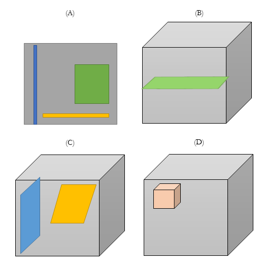
Figure 4. Subsetting multidimensional arrays

Figure 4A is an example of some of the extractions possible from a 2d image. It is possible to select a pixel, a defined portion, or an entire row (yellow) or column (blue) from the larger array. For geospatial applications, subsetting operations are likely to include the selection of region from a larger image (e.g.,  Colorado from the entire US National Landcover Dataset) (Figure 4A green). Subsetting in higher dimension is also possible (Figure 4B and 4C). A plane of data on any axis can be subsetted from a 3dimensional array. For geospatial applications, using Hagestrand’s Time Geography paradigm, this is typically thought of as space-time cubes, and the planar subsets are space and time specific (Hedley, 1999; Miller, 1991). Additionally, smaller space-time cubes could also be generated from larger space-time cubes (Figure 4D).

2.2.2 Filtering

Filter operations are a heavily used feature in Database Management Systems (DBMS). A filter operation will retain only the values of interest from a particular array. Filter operations are analogous to the WHERE clause in a relational database. 

2.2.3 Aggregation

Aggregation operations are another feature that exists in RDMB that exist in Array Databases. Aggregations in RDBM allow for the summarize information by columns over tables. Array Databases expand this concept a further, by summarizing values/columns and by dimensions. For geospatial, performing aggregations by dimensions may not be immediately useful or intuitive. However, summarizing information by a single geographic dimension provides insight into how values change across one dimension of space.

2.2.4 Joins

Another feature implemented in Array Databases are joins. Joins in relational databases require two tables to have field/columns with the same values. Joining two related tables allows information to be linked together and relational databases are known for the flexibility of their joins (i.e., inner, right, left, full) and their ability to join multiple tables and join large datasets (Mishra & Eich, 1992). Array databases support a limited set of joins (i.e., cross join, inner join). A join in an array database is not performed on the attributes, but the dimensions of the array. For example, Figure 5 demonstrates the join between two 2d arrays.  Therefore pixel value 5 at (0,0) in array1 will now be aligned with pixel value 80 at (0,0) in array2. The result of any join operation is a new array with two fields/columns. The resulting array can have additional array operators applied to it as well.

Figure 5. Array to Array Join

3. Spatial Analysis for Array Databases

The ability to apply raster operations (local, focal, and zonal) within an array database is a primary motivation for placing geospatial data within an array-store database. The ability to apply all rasters operations within these environments is an active area of research.

3.1 Local Operators

Local raster operations are a class of operations characterized by performing an operating on each cell individually without reference to the surrounding cells. Many geospatial local operations have implemented on these platforms, such as reclassification, histogram, and map algebra, though they are likely to use other names within each platform. A benefit of performing these operations within these platforms is that the data is already partitioned and therefore can be operated on with independent parallel operations. Camara and colleagues (2016) provide specific documentation on the geospatial operations for SciDB. 

3.2 Focal Operators

Focal operators differ from local operators in that the output values are influenced by surrounding cells. Both RasDaMan and SciDB allow a kernel or window to be defined by any arbitrary size and in multiple dimensions. The value of a particular cell is determined by the aggregate operation used within the kernel.

3.3 Zonal Operators

Zonal operations are complex analyses for array databases as they typically involve both raster and vector datasets. Vector data types are not natively supported in array stores. Therefore, to conduct a zonal analysis, the vector dataset must be rasterized and loaded into the array database for analysis. Even after the data is loaded their complexity does not diminish, because zonal operations are loosely-synchronous (Ding & Densham, 1996). Therefore, when a calculation is applied to a specific zone, the entire dataset is not affected. Zonal operators like polygonal summaries are possible in array database, but require join and aggregation operators (Haynes, Manson, & Shook, 2017).

4. Future Directions

Array Databases are a major innovative tool in the GIScience toolbox. The ability to manipulate, edit, and analyze big spatial data at scale is a tremendous advantage for any researcher using multidimensional raster data. The advantage of using an array database is that the researcher no longer needs to construct a parallel environment that performs operations across the data (e.g., moving data to the computation). Instead, the data and the parallel processing framework are in the same location (e.g., moving the computing to the data). This allows any algorithms developed using the computation framework to be implemented in parallel with no additional expertise.

A major barrier that exists for array databases is the challenge of loading data into the system. Currently, only RasDaMan and Google Earth Engine (GEE) natively support reading of geospatial satellite imagery. GEE is the first platform to natively support reading of all datasets supported by the Geographic Data Abstraction Library (GDAL), whereas RasDaMan currently only supports four image formats (i.e., Tagged Image File Format, Portable Network Graphics, Joint Photographic Experts Group, and Digital Elevation Model). The SciDB community has created an extension for GDAL that convert any GDAL read dataset into SciDB format (Appel, 2017). An active area of ongoing research is the development of tools to read and export spatial data into the database (Kovanen, Makinen, & Sarjakoski, 2018).

The sudden increase in production and availability of big raster data presents a tremendous opportunity for the GIScience community. Geospatial data has always been large, but now we are at a critical time in which spatial data is available in the spatial and temporal granularity to answer critical questions about the environment and human interaction. The development of spatial infrastructures is necessary to support this production of new knowledge, as well as, facility that transition away from the reliance on the computational capacity of their workstations to cloud or grid computing environments. The development of combined spatial data and big computation infrastructures like array databases are the future in which analyses on big data are performed in parallel and disseminated.

References

- Abadi, D. J., Boncz, P. A., & Harizopoulos, S. (2009). Column-oriented database systems. Proceedings of the VLDB Endowment, 2(2), 1664-1665.
- Appel, M. (2017). SciDB4GDAL [Github]. Retrieved March 1, 2019, from SciDB4GDAL website.
- Baumann, P. (2016). A voyage through dimensions: Recent innovations in geospatial coverages. 2016 IEEE International Geoscience and Remote Sensing Symposium (IGARSS), 3599–3601.
- Baumann, P., Dehmel, A., Furtado, P., Ritsch, R., & Widmann, N. (1998). The Multidimensional Database System RasDaMan. ACM Sigmod Record, 27(2), 575-577.
- Baumann, P., Misev, D., Merticariu, V., Huu, B. P., Bell, B., & Kuo, K.-S. (2018). Array Databases: Concepts, Standards, Implementation. Journal of Big Data 8, 28.
- Buck, J. B., Watkins, N., LeFevre, J., Ioannidou, K., Maltzahn, C., Polyzotis, N., & Brandt, S. (2011). SciHadoop: array-based query processing in Hadoop. Proceedings of 2011 International Conference for High Performance Computing, Networking, Storage and Analysis on - SC '11, 1.
- Camara, G., Assis, L. F., Ribeiro, G., Ferreira, K. R., Llapa, E., & Vinhas, L. (2016). Big earth observation data analytics: matching requirements to system architectures. Proceedings of the 5th ACM SIGSPATIAL International Workshop on Analytics for Big Geospatial Data - BigSpatial '16, 1-6.
- Ding, Y., & Densham, P. J. (1996). Spatial strategies for parallel spatial modelling. International Journal of Geographical Information Systems, 10(6), 669-698.
- Haynes, D., Manson, S., & Shook, E. (2017). Terra Populus' Architecture for Integrated Big Geospatial Services. Transactions in GIS, 21(3), 546-559.
- Hedley, N. R., Drew, C. H., Arfin, E. A., and Lee, A. (1999). Hagerstrand revisited: Interactive space-time visualizations of complex spatial data. Informatica, 23(2), 155-168.
- Kersten, M., Zhang, Y., Ivanova, M., & Nes, N. (2011). SciQL, a query language for science applications. AD '11: Proceedings of the EDBT/ICDT 2011 Workshop on Array Databases, 1–12.
- Kini, A., & Emanuele, R. (2014). Geotrellis: Adding Geospatial Capabilities to Spark.
- Kovanen, J., Makinen, V., & Sarjakoski, T. (2018). An Approach for Assessing Array DBMSs for Geospatial Raster Data. GEOProcessing, International Conference on Advanced Geographic Information Systems, Applications, and Services, 6.
- Marques, P. J. P. (1998). Arbitrary Tiling Of Multidimensional Discrete Data Cubes In The RasDaMan System (Bavarian Research Center for Knowledge-Based Systems).
- Miller, H. J. (1991). Modelling accessibility using space-time prism concepts within geographical information systems. International Journal of Geographical Information Systems, 5(3), 287-301.
- Mishra, P. & Eich, M. H. (1992). Join processing in relational databases. ACM Computing Surveys (CSUR), 24(1), 63-113.
- Pavlo, A., Curino, C., & Zdonik, S. (2012). Skew-aware automatic database partitioning in shared-nothing, parallel OLTP systems. Proceedings of the 2012 ACM SIGMOD International Conference on Management of Data, 61-72.
- Planthaber, G., Stonebraker, M., & Frew, J. (2012). EarthDB: scalable analysis of MODIS data using SciDB. Proceedings of the 1st ACM SIGSPATIAL International Workshop on Analytics for Big Geospatial Data, 11-19.
- Stonebraker, M. (1986). The Case for Shared Nothing. IEEE Database Eng. Bull., 9(1), 4-9.
- Stonebraker, M., Brown, P., Poliakov, A., Raman, S. (2011). The Architecture of SciDB. In: Bayard Cushing, J., French, J., Bowers, S. (eds) Scientific and Statistical Database Management. SSDBM 2011. Lecture Notes in Computer Science, vol 6809. Springer, Berlin, Heidelberg.
- Wang, W., Liu, T., Tang, D., Liu, H., Li, W., & Lee, R. (2016). SparkArray: An Array-Based Scientific Data Management System Built on Apache Spark. 2016 IEEE International Conference on Networking, Architecture and Storage (NAS), 1-10.
- Wang, Y., Jiang, W., & Agrawal, G. (2012). SciMATE: A Novel MapReduce-Like Framework for Multiple Scientific Data Formats. 2012 12th IEEE/ACM International Symposium on Cluster, Cloud and Grid Computing (Ccgrid 2012), 443-450.
- Widmann, N., & Baumann, P. (1999). Performance evaluation of multidimensional array storage techniques in databases. Proceedings. IDEAS'99. International Database Engineering and Applications Symposium (Cat. No.PR00265), 385-389.
Learning outcomes
-
101 - Compare and contrast the conceptual differences between an array database store and a relational database.
Compare and contrast the conceptual differences between an array database store and a relational database.
471 - Describe related platforms (e.g., SQL, Hadoop, Apache Spark) that implement array data models.
Describe related platforms (e.g., SQL, Hadoop, Apache Spark) that implement array data models.
506 - Describe the basic spatial operations of array stores.
Describe the basic spatial operations of array stores.
597 - Describe the multi-dimensional model and the basic operations available for array data stores.
Describe the multi-dimensional model and the basic operations available for array data stores.
740 - Differentiate between array-store, column-store, and row-store databases.
Differentiate between array-store, column-store, and row-store databases.
1097 - Explain the approach used for storing and structuring data in array databases.
Explain the approach used for storing and structuring data in array databases.