[DC-04-012] Fundamentals of Aerial Photo Interpretation

Myint, S. (2024). Fundamentals of Aerial Photo Interpretation. The Geographic Information Science & Technology Body of Knowledge (2023 Version), John P. Wilson (Ed.). DOI: 10.22224/gistbok/2024.1.4

1. Elements of Image Interpretation
2. Airphoto Interpretation Key
3. Scale of an Aerial Photograph
4. Basic Concepts of Aerial Photographs
5. Land Use / Land Cover Classification and Mapping

 

1. Elements of Image Interpretation

Sensors or cameras mounted to aircraft and satellites are called airborne sensors or cameras and spaceborne sensors or cameras respectively. This chapter deals with the interpretation of data produced mainly by airborne sensors. There are two types of aerial photographs that are available – digital and hard copy, and almost all modern data are made in digital format. However, the principles between the two are fundamentally the same, with the difference being pixels stored in a computer versus silver-halide crystals suspended in an immersion (hard copy photo).

When we can correctly identify what we see on the aerial photographs, transform them into information (e.g., map, tables, statistics), and transfer this information to others, we are practicing airphoto interpretation. An aerial photograph contains raw photographic data. These data become usable information when they are processed by a human interpreter through an appropriate and sensible interpretation.

It is conventional to use principles of aerial photo interpretation that has been developed for more than 175 years (Estes et al., 1983; Schott, 2007; Jensen, 2013; Lillesand et al., 2015). The most important aspect of these principles are the elements of airphoto interpretation. These elements include location, size, tone, site, shape, shadow, texture, pattern, height and depth, situation, and association.

1.1 Tone refers to the relative darkness or level of brightness of objects and features on aerial photographs. For example, cement parking lot or sandbar is light or bright, whereas swamp is dark. It is possible to distinguish between deciduous and coniferous forests on black and white infrared photographs using their differences in reflected energy that show relative brightness or darkness. It can also be referred to as the color of a photo. 

1.2 Shape is the outlined of each object, general form, or configuration. In the case of stereoscopic photographs, the object’s height also define its shape. For example, soccer fields with running tracks and baseball fields have very distinct shapes.

1.3. Texture is the frequency of tonal change or characteristic arrangement of repetitions of tone or color on the photographic image. It is a combined effect of insignificant features that could be too small to be identified individually on an aerial photograph. Texture is generated by an aggregation of their tiny individual shape, size, pattern, shadow, and tone. It represents the overall visual smoothness or coarseness of image features.

1.4. Shadows are important to interpreters in two aspects: (1) the shape or outline of a shadow gives an impression of the possible objects which helps photo interpretation and (2) determination of relative heights of objects or accurate measurements of object heights. However, objects within shadows reflect little or no light, and it is a challenging task to discern these objects on aerial photos.

1.5. Site refers to geographic location of an object (e.g., x and y coordinates). It could also be related to elevation, slope, aspect, proximity to identifiable objects and features (roads, water, agriculture, utilities). For example, certain tree species or a type of forest would grow above a certain elevation (e.g., coniferous forest) whereas other tree species occur on coastal areas that are periodically submerged by tides (e.g., mangroves).

1.6. Association is the occurrence of certain features or objects relative to other features or objects. For example, universities are normally found in association with a football stadium with large parking lots. Some might argue that association is somewhat related to site. Site is related to geographic location whereas association is connected to relative location.

1.7. Pattern relates to spatial configuration of objects and features. The repetition of certain objects and features show some type of forms that are recognizable as a whole. Their spatial arrangements or relationships defines characteristic of many objects together, both natural and engineered features. This arrangement gives objects a pattern that help the aerial photo interpreter in identifying them.

1.8. Size is defined as the area extent of objects on aerial photographs that need to be considered in connection to the photo scale. E.g., A small office building might be misinterpreted as a shopping mall if size was not considered with regard to scale. Sometimes the interpreter needs to consider relative sizes among objects on the same photograph or different photographs of the same scale.

1.9. Spatial resolution or scale is related to object size, shape, shadow, or pattern. It is especially important if an interpreter attempts to determine the size of an object. It always gives a applicable limit on interpretation because some objects are too small or have too little contrasts with their surroundings to interpret.

1.10. Time of acquisition is an important factor in identifying some features and objects. For example, school parking lots may be busy between 7 am and 3 pm on school days whereas parking lots of office buildings may be packed between 9 am and 5 pm. Another example is the planting and harvesting times of different crops are different, and it can potentially enable the interpreter to accurately identify different crops. It is also possible for us to distinguish between deciduous and coniferous forests in photos acquired in winter since deciduous trees shed leaves in winter.

Figure 1 demonstrates most of the elements of image interpretation described above.

 

2. Airphoto Interpretation Key

It is customary to use an airphoto interpretation key to evaluate objects and features presented on photographs in an organized and consistent manner. It provides a step by step procedure or guidance to correctly identify features and objects. There are two general types of airphoto interpretation keys available.

2.1. Selective key: contains numerous samples of photos or pieces of photo examples with comprehensive descriptions and explanations. The interpreter identifies or interprets objects and features on photos that most closely resembles the feature or condition in the selective key.

2.2. Elimination key: This type of interpretation key consists a step by step procedure from the general to the specific that enables the interpreter to eliminate all features or objects except the one being identified. Elimination keys generally comes in the form of dichotomous keys, and the interpreter makes a series of selections between two options at a time until the final class is determined.

The use of elimination keys can be expected to give more affirmative outcomes than selective keys. However, it can also lead to inaccurate classification and identification when the interpreter is forced to make a decision between two unaccustomed or unusual choices of image properties.

The selective key describes and explains objects or classes of phenomena in detail, and the image interpreter has to select the closest fit for a particular object or feature of interest. This type of key is restricted by the level of detail which can be handled by means of the selective key. The selective key is best used when the interpreter is genuinely aware of the characteristics of objects and classes to be identified in connection to the elements of image interpretation.

On the other hand, elimination keys are handled step by step through an array of possible identifications, and the interpreter is pushed to reject all incorrect choices at each step. This approach is best used when the interpreter does not have a local area knowledge and is not aware of objects and features to be identified. This type of key is effectively used when the keys completely cover all possible objects and features in the photo. However, it may not be possible to cover all possible objects and features in a particular area.

It should also be noted that no one key will handle all jobs incidental to the effective interpretation of aerial photographs. It is recommended that both keys are employed to perform an airphoto interpretation if at all possible.

Figure 2 shows an example of a dichotomous key prepared for the selection of some tree species and fruits or orchards. This hypothetical example was created to demonstrate how dichotomous keys generally function to determine different vegetation categories. But this example does not represent any particular tree species or fruit trees. Please note that this example shows how the interpreter can select 6 different tree species. In the real-world situation, there could be far more than six tree species in a particular region or study area.

 

3. Scale of an Aerial Photograph

There are basically two types of scale – (1) map scale, (2) photo scale.

3.1. Map scale is defined as the ratio of a particular distance on a map to the corresponding distance on the ground.

3.2. Photo scale: Similarly, the scale of a an airphoto is the ratio of a distance on the photo to the corresponding distance on the ground.

Since a map is geometrically corrected using a map projection to represent location of each point in a map as accurately as possible in comparison to the ground location of corresponding points, map scale is not affected by varying terrain heights in a particular area. Since an airphoto is a perspective projection, its scale varies with changes in terrain elevation.

Map scale = a'b'/AB

where a'b' = map distance; AB = corresponding ground distance.

Photo scale = ab/AB

where ab = photo distance; AB = corresponding ground distance.

 

An aerial photo scale may be described as unit equivalent, unit fraction, representative fraction, or ratio. 

• Unit equivalents: 1 cm = 100 m
• Unit fraction: 1 cm / 100 m
• Representative fraction: 1/10,000
• Ratio: 1:10,000

 

 

3.3. Photo scale of a vertical photograph over flat terrain
There is almost no scale variation across an airphoto if it is a perfect vertical photo taken over a complete flat terrain without any objects on the ground. It is practically impossible to obtain a vertical photo acquired over an area without variation in terrain elevation and object heights above the ground. It should also be noted that any objects standing above the terrain lean away radially from the center of the photo, called principal point. In the above statement, it is true only if there is no object above or below a selected datum (flat terrain).

 

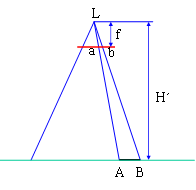
From 

where

• S = scale
• AB = ground distance
• ab = photo distance
• f = focal length, and
• H ´ = flying height.

 

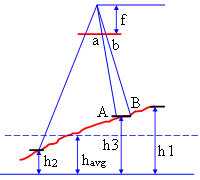
3.4. Scale of a vertical photograph over variable terrain
If the terrain elevation varies across an area covered by an airphoto, the photo scale will similarly vary.

The denominator H - h is the flying height above a particular terrain point. There are an infinite number of scales if an airphoto is taken over an area with varying terrain elevations. This is one of the fundamental differences between an aerial photograph and a map. An orthophoto or orthophotograph is an airphoto that is geometrically corrected with a particular map projection so that the scale is constant across space. It is an accurate representation of the Earth’s surface that is precisely adjusted for topographic variations.

3.5 Average Photo Scale

It is a common practice to use an average photo scale to represent the overall mean scale of a vertical photograph taken over different terrain elevations. An average photo scale is the scale at the average elevation of the terrain covered by a particular photograph and is expressed as

 

 

3.6. Other methods of determining scale of vertical photographs
We have learned how the scales of vertical airphotos are calculated in terms of camera focal length, flying height, and terrain elevation in the previous sections. However, there are other approaches of scale calculation which do not require these measurement values. If we know the distance on an airphoto and the corresponding distance on a map with a known map scale.

 

4. Heights, Distances, and Areas of Objects in a Vertical Aerial Photo

It is a common practice that the photo interpreter estimates heights, distances, and areas of objects and features in a vertical airphoto using different methods.

4.1. Basic concepts of aerial photographs
There are some fundamental concepts of aerial photographs that the photo interpreter needs to know in order to compute the heights, distances, and areas of objects in a vertical airphoto. The following paragraphs present definitions of some important concepts and terms used in airphoto interpretation.

Principal point (PP): the intersection of the camera optical axis and the photo plane (center of an air photo).

Conjugate principal point: the points identified on an airphoto that are transferred from the image centers of the preceding and succeeding airphotos.

Flight axis: A line drawn through the principal points and the conjugate principal points.

Nadir: a point in an airphoto directly below airplane at time of photo (Nadir point is the same as principal point (PP) for vertical photos).

Nadir-line: The line traced on the ground directly beneath the aircraft during acquisition of aerial photos or a line connecting nadir points is called the nadir line.

Flight lines: aerial photos are normally taken along a series of parallel passes called flight lines or flight strips. An example of photographic coverages along two adjacent parallel flight lines is shown in Figures 6 and 7.

Stereoscopic overlap area: The area coverage common to an adjacent pair of photographs in a flight strip is called the stereoscopic overlap area where you can see 3D view under either a mirror stereoscope or pocket stereoscope.

Image mosaic: A mosaic is obtained by assembling together the individual photographs into a single continuous image.

Endlap or forwardlap: Each photograph in the line of flight covers an area that overlaps the area covered by the previous photographs by about 55%-65%, called endlap or forwardlap. This overlapping area between two adjacent photos is the area that is used to see 3D view of an area of interest.

Side lap: Adjacent flight lines are used to take a series of parallel photos so that there is also a sideway overlapping portion of adjacent strips, called side lap, usually 30%. This part of the photo pairs is not used for a stereoscopic view of the image.

A block of photos: The photographs of two or more sidelapping strips used to cover an area is referred to as a block of photos

Stereopairs: Stereoscopic coverage is created by adjacent pairs of overlapping airphotos called stereopairs.

 

 

 

Air base: The ground distance between the two adjacent photo centers at the time of exposure is referred to as air base.

Vertical exaggeration: The ratio between the air base and the flying height above ground is called vertical exaggeration. The higher the base height ratio, the greater the vertical exaggeration perceived by airphoto interpreters (Figure 8). It should be noted that vertical exaggeration is only relevant for optical stereo viewing, and digital photogrammetry does not have any serious issue regarding vertical exaggeration.

 

 

4.2. Relief displacement on a vertical airphoto to determine object height

Relief displacement is the apparent shift in the position of an image caused by the height of the object, i.e., its elevation above or below a selected datum. Relief displacement is caused any object standing above the terrain to lean away radially from the principal point of an airphoto. Figure 9 shows the relief displacement of an object standing above the ground.

 

 

From similar triangles A A' A" and LOA"

Replacing distances D and R with d and r at the scale of the photo, we obtain

• h = height above datum of object point whose image is displaced
• H = flying height above same datum selected for h
• D = relief displacement that can be measured on an airphoto
• R = radial distance on photograph from principal point to displaced image.
• Note: The units of d and r have to be the same.

If we know the photo scale, we can measure the photo distance and convert it to ground distance using the scale formula mentioned earlier.

H´ = Flying height; f = Focal length; AB = Ground distance; ab = Photo distance. 

4.3. Stereoscopic parallax on a vertical airphoto to determine an object height

The change in position of an object from one photograph to the next overlapping photograph affected by the aircraft's motion is termed stereoscopic parallax or simply parallax. Parallax exists for all objects appearing on adjacent pairs of overlapping airphotos called stereopairs. Figure 10 shows overlapping airphotos of a terrain point T with height hA.

From similar triangles    we have  

From similar triangles   , we have

4.4. Area Measurement

There are different types of area measurements on aerial photographs. The accuracy of area measurement depends not only on the variation in terrain elevation but also on the measuring device used. Large errors in area measurements can be found even with vertical photos in areas of medium to high elevations. Hence, accurate measurements can be made on large scale vertical photos taken on a flat terrain. A simple scale formula can be used to measure the area of linear shaped features, especially made by humans. For example, the area of a parking lot can be obtained by measuring it width and length on the photo and converting to ground distances. The area of a circular feature can be obtained after measuring its radius. There are some methods to measure the area of irregularly shaped features on a photo.

One of the straightforward approaches to measure the area of irregularly shaped features on a photo is to use a transparent grid overlay consisting of rectangles or squares of known area. The interpret place the transparent grids over the airphoto and the area of a particular feature or an object is estimated by counting number of grids that fall within the feature or object to be measured. A more commonly used method uses a grid overlay transparency with dot grids that are uniformly placed dots. The interpreter superimposes the dot grid sheet over the airphoto and counts the number of dots falling within the desired region. Since there is a conversion table that shows number of dots and area coverage, the photo area of the object or feature can be determined.

 

5. Land Use / Land Cover Classification and Mapping

Land use land cover types of a particular area in the form of a classified map is crucial for various planning and management, sustainable development, policy formulation, finding solutions, and answering science questions. It is widely considered a vital component for modeling and understanding the changing climate and earth system (Jensen, 2013).

5.1. Classification refers to a type of categorization of remotely sensed data using spectral, spatial, and temporal resolution.

Land cover is defined as the type of features present on the earth surface. Trees, grass, ponds, lakes, concrete parking lot, and concrete highways are all examples of land cover types. 

Land use refers to the human activity or economic function that has been taken place in a specific portion of land. For example, a particular section of an urban area may be used for single or multiple family residential type. The same portion of land would have a land cover consisting of roofs, asphalt roads, sidewalks, driveways, grass, shrubs, and trees. Its land use could be described as single family or multiple residential use.

The United States Geological Survey (USGS) developed a system for identifying land use and land cover classes from remotely sensed data (Anderson et al., 1976). Even though the system was developed in the mid-1970s, the key concept, basic definitions, general organizations, and structure are still compelling and appropriate to various remote sensing classification at different level of scales today. There are more land use land cover classification systems developed according to the level of details demanded, nontraditional categories to be extracted, or their distinctive needs. However, these systems have been developed based on the basic foundation of the USGS land use land cover classification system and still follow the concept and structure of the USGS system. Many of the recent classification systems are purely minor adjustments and alterations of the original USGS system to meet specific needs (Jensen, 2013).

The following criteria were used to developed the USGS land use and land cover classification system (Anderson et al., 1976).

1. The minimum level of interpretation accuracy using remotely sensed data should be at least 85%.
2. The accuracy of interpretation for the several categories should be about equal.
3. Repeatable or repetitive results should be obtainable from one interpreter to another and from one time of sensing to another.
4. The classification system should be applicable over extensive areas.
5. The categorization should permit land use to be inferred from the land cover types.
6. The classification system should be suitable for use with remote sensing data obtained at different times of the year.
7. Categories should be divisible into more detailed subcategories that can be obtained from large scale imagery or ground surveys.
8. Aggregation of categories must be possible.
9. Comparison with future land use and land cover data should be possible.
10. Multiple uses of land should be recognized when possible.

The USGS definitions for Level 1 land use land cover classes (Anderson et al., 1976) are presented in the following paragraphs. The descriptions of individual land use land cover classes at Level 2 are provided in Anderson et al. (1976) but are not discussed here.

Urban or built-up land: is comprised of cities; towns; villages; strip development along highways; transportation; power; and communication facilities; and areas such as those occupied by mills, shopping centers, industrial and commercial complexes, and illustrations that may, in some instances, be isolated from urban areas. This category takes precedence over others when the criteria for more than one category are met. For example, residential areas that have sufficient tree cover to meet forest land criteria should be placed in the residential category.

Agricultural land: may be broadly defined as land used primarily for production of food and fiber. The category includes the following uses: cropland and pasture, orchards, groves and vineyards, nurseries and ornamental horticultural areas, and confined feeding operations. Where farming activities are limited by soil wetness, the exact boundary may be difficult to locate and agricultural land may grade into wetland. Similarly, when wetlands are drained for agricultural purposes, they are included in the agricultural land category.

Rangeland: historically has been defined as land where the potential natural vegetation is predominantly grasses, grass like plants, forbs, or shrubs and where natural herbivory was an important influence.

Forest lands: have a tree-crown areal density (crown closure percentage) of 10% or more, are stocked with trees capable of producing timber or other wood products, and exert an influence on the climate or water regime.

Water: The delineation of water areas depends on the scale of data presentation and the scale and resolution characteristics of the remote sensor data used for interpretation of land use and land cover. (Water as defined by the Bureau of the Census includes all areas within the land mass of the United States that persistently are water covered).

Wetlands: are those areas where the water table is at, near, or above the land surface for a significant part of most years. The hydrologic regime is such that aquatic or hydrophytic vegetation is usually established, although alluvial and tidal flats may be non-vegetated.

Barren land: is land of limited ability to support life and in which less than one-third of the area has vegetation or other cover. This category includes dry salt flats, beaches, bare exposed rock, strip mines, quarries, and gravel pits.

Tundra: is the term applied to treeless regions beyond the limit of the boreal forest and above the altitudinal limit of trees in high mountain ranges.

Perennial snow or ice: Certain lands have a perennial cover of either snow or ice because of a combination of environmental factors that cause these features to survive the summer melting season. In so doing, they persist as relatively permanent features on the landscape and may be used as environmental surrogates.

USGS land use land cover classification system for level 1 and 2 is provided in Table 1. An example aggregation of land use/land cover types is presented in Figure 11.

 

Table 1. USGS Land Use/Land Cover Classification System for Use with Remote Sensing Data (Level 1 and 2) (Anderson, et al., 1976). 

Level 1	Level 2
1 Urban or built-up land	11 Residential
	12 Commercial and service
	13 Industrial
	14 Transportation, communications, and utilities
	15 Industrial and commercial complexes
	16 Mixed urban or built-up land
	17 Other urban or built-up land
2 Agriciultural land	21 Cropland and pasture
	22 Orchards, groves, vineyards, nurseries, and ornamental horticultural areas
	23 Confined feeding operations
	24 Other agricultural lands
3 Rangeland	31 Herbaceous rangeland
	32 Shrub and brush rangeland
	33 Mixed rangeland
41 Forest land	41 Deciduous forest land
	42 Evergreen forest land
	43 Mixed forest land
5 Water	51 Steams and canals
	52 Lakes
	53 Reservoirs
	54 Bays and estuaries
6 Wetland	61 Forested wetland
	62 Nonforested wetland
7 Barren land	71 Dry salt flats
	72 Beaches
	73 Sandy areas other than beaches
	74 Bare rock exposed
	75 Stripmines, quarries, and gravel pits
	76 Transitional areas
	77 Mixed barren land
8 Tundra	81 Shrub and brush tundra
	82 Herbaceous tundra
	83 Bare ground tundra
	84 Wet tundra
	85 Mixed tundra
9 Perennial snow or ice	91 Perennial snow fields
	92 Glaciers

 

 

Table 2. Example Representative Image Data for different Land Use/Land Cover Classification Levels (Anderson, et al., 1976; Lillesand, et al., 2015).

Land Use / Land Cover Classification Level	Relevant Remotely Sensed Data for Interpretation
I	Low to moderate resolution satellite data (e.g., Landsat MSS data)
II	Small-scale aerial photographs; moderate resolutoin satellite data (e.g., Landsat TM data)
III	Medium-scale aerial photographs;  high resolution satellite data (e.g., data acquired by commercial high resolution systems)
IV	Large-scale aerial photographs

References

- Anderson, J. F., Hardy, E. E., Roach, J. T., and Witmer, R. E. (1976). A Land Use and Land Cover Classification System for Use with Remote Sensor Data. Geological Survey Professional Paper No. 964, U.S. Government Printing Office, Washington DC, 28.
- Estes, J. E., Hajic, E. J., Tinney, L. R. (1983). Fundamentals of image analysis: Analysis of visible and thermal infrared data, Manual of Remote Sensing, R. N. Colwell, Ed., Falls Church, VA: American Society of Photogrammetry, 1:1039-1040.
- Jensen, J. R. (2013). Remote Sensing of the Environment: An Earth Resource Perspective. 2nd Edition, Pearson Prentice Hall, Upper Saddle River, 618 pp.
- Lillesand, T. M., Kiefer, R. W., & Chipman, J. W. (2015). Remote Sensing and Image Interpretation (7th Edition). Hoboken, NJ: John Wiley.
- Schott, J. R. (2007). Remote Sensing: The Image Chain Approach, 2nd Edition, Oxford: Oxford University Press, 688 pp.
Learning outcomes
-
543 - Describe the differences between oblique and vertical aerial photographs.
Describe the differences between oblique and vertical aerial photographs.
982 - Explain about why aerial photographs are orthorectified.
Explain about why aerial photographs are orthorectified.
1197 - Explain the relevance of the concept "parallax" in stereoscopic aerial imagery
Explain the relevance of the concept "parallax" in stereoscopic aerial imagery
1215 - Explain the various distortions found in vertical aerial photographs.
Explain the various distortions found in vertical aerial photographs.
1662 - Use photo interpretation keys to interpret features on aerial photographs
Use photo interpretation keys to interpret features on aerial photographs