[AM-05-076] Network Route & Tour Problems in Geographic Information Systems

Roy, A. (2024). Network Route and Tour Problems in Geographic Information Systems.  The Geographic Information Science & Technology Body of Knowledge (2024 Edition). John P. Wilson (Ed.). DOI: 10.22224/gistbok/2024.1.22. 

1. Definitions
2. Defining a Network Mathematically
3. Cost Matrix of a Network Graph
4. Shortest Path Algorithm
5. Applications of Spatial Networks
6. Other Algorithms

1. Definitions

To begin with the understanding of network analyses we need to get a hold of a few key terms that need to be defined early on:

1. Nodes/Vertices: Intersections or junctions within a network that is a placeholder for an amenity for example - a hospital, a fire station or a school. In graph theory these nodes are termed as vertices.
2. Edges: The connections between the nodes which establish a pathway is defined as an edge. Edges are exemplified by means of their interconnections to several or just one node. For example: The streets in a city are considered edges, connecting it to the nodes will mean the route that connects a home to an amenity such as a hospital or a school where home and hospital are nodes and the streets connecting these nodes are edges.
3. Connections: The interconnectivity established by several nodes and edges are called connections. These connections are relevant in understanding the essence of choice in a network routing problem. The more the connections to a node, the higher its importance in a network. Such connections are also ranked higher in a network setup.
4. Weights: The values associated with the impedance or cost of connections around a node are distributed across the edges as weights. For example, if a connection takes 20 minutes to reach from node A to node B and node C to node B takes only 15 minutes, the second connection is preferred as the travel time associated as weight to each connection can be compared and ranked in order of preference.
5. Distances: In a network-based system distances are usually measured in network distances. Sometimes the weights can also represent distance between nodes. If the distance is not a network distance it is measured in regular units like km, m, miles etc. For example, in a traffic network context, the distance could either be measured in units of time such as time to destination or in miles such as 5 miles to the destination etc.
6. Flows: The flow within a network is an interesting piece to the puzzle. When we are defining the nodes and edges of a network along with the weights associated to each edge, we usually assume the flow between a pair of nodes along the edge is bidirectional meaning that if A and B are connected nodes in a traffic network, vehicles will travel both from A to B and B to A. For unidirectional networks there is a limitation that the flow is either restricted from A to B or from B to A for example in a hydrological network setup where water flows along the slope only in a single direction. The network/graph will be called an undirected network/graph or a directed network/graph based on whether or not flows are directional from an origin to a destination or ceteris peribus.
7. Network: The entire concept of nodes, edges, connections, distance measures and flows culminate in the definition of a single network. A network is therefore a system that is defined through a connected set of nodes which has a system of flow defined through the connections by means of its edges each of which have associated weights and possibly a direction of flow.

2. Defining a Network Mathematically

The structure of a street network is the most common example of a city’s network. It shows the origin and destination of a trip for example riding a bicycle and the direction of the flow from the origin to the destination. In Figure 1 we can see the network route of a bicyclist’s travel trajectory from the origin (City of Irvine Civic Center) to the destination (San Marino Park) with the total distance travelled, modality of travel (bicycling) used and the travel time which is shown in dark blue line.

An alternative path highlighted in a lighter shade of blue is also suggested along the same OD-flow. It is up to the discretion of the user of an application that suggests the optimal route or the bicyclists to choose between Path 1 (6-minute trip) or Path 2 (5-minute trip). In this particular use case, the time difference is a simple 1 minute of lag but in vehicular traffic the temporal gains and losses would matter quite a lot. For example, in case of freights and heavy vehicles such as trucks the choice of route depends a lot upon the long route choices a driver must make while delivering logistical supplies. The decision of saving time over distance then becomes crucial and a complex problem.

To understand the network structure in a bit more detail let us represent the network as a mathematical graph G (Figure 2) with vertices/nodes V and edges E. Therefore, the graph is now structured mathematically as G = (V, E), let the vertices be numbers so; V = {1,2,3,4,5} and the edges be considered as: {{1,2}, {2,3}, {1,5}, 3,1}, {3,5}, {1,4}, {2,4}, {4,5}, {5,2}}.

The concept of networks is in essence a shared idea of a systems-based approach wherein planners think of cities and societies as a single operational system and interact with each other in ways not just culturally but with exchange of commodities, movement of goods/supplies and jobs. The socio spatial connection ties these systems of communications together thereby formulating a network structure. The behavior of such interconnected systems manifests themselves in modes of transportation, movement of people and exchange of ideas that help to theorize the economic structure of the networked system and in case of movements, the entropy of the system based on its complexity – whether be it the road structures or availability of vehicle ownership.

The networks once interconnected pose a unique problem of optimizing transportation flows and energy exchange across different socioeconomic domains. Thus, the necessity for routing problems or shortest path approach emerges from an operations research concept using matrix operations in the discrete system. However, when the theorizing of these systems summarizes a surface rather than a route/path, the objective function becomes a cost function that can derive a least cost surface that preserves entropy and connects efficiently/optimally.

3. Cost Matrix of a Network Graph

Let us imagine a graph G which is a network of nodes and edges. The network G is now a directed graph with nodes and edges connected from several origins to several destinations. We can mathematically represent the edges as E = {(I,j)} which are a set of directed networks. Now we can define and adjacency matrix for G based on the connections among the nodes/vertices V as per the edge definitions in E.

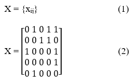
Now let us suppose each edge E had an associated time cost (i.e., a travel time in minutes) along the network flows. We could easily create a cost matrix Cij for the network G as:

In equation (3) the cost tends to infinity when the nodes are not present in the adjacency matrix. The diagonal elements of the adjacency matrix (Eqn 2) is by default set to zero as there is no flow of traffic/bicyclists if the node is one and the same as no movement literally happens in that scenario. In reality, the nodes in a street network are mostly connected to other nodes/street intersections that are geographically proximal to a specific node. For example, 13th Street cannot have a direct connection to 1st street without flowing through the network in a grid-designed city street network.

4. Shortest Path Algorithm

The value of a network lies in optimizing how fast a traveler can be transported from origin ‘i’ to a destination ‘j’ with reduced time and computational cost of solving for the shortest path. The original version of the shortest path problem was developed by Dijkstra in 1959 (Dijkstra, 1959). It has been reused in several transportation and congestion solving applications ever since but the problem in itself has a polynomial time solution and has a worst case solving complexity of 

Let us algorithmically define the shortest path algorithm for a directed network N = (V,E) with vertices V and edges E and weights  for each (i,j)  ∈E as follows:

Step 1: Set the initial distance to each vertex Vi,j a tentative distance value. Let the starting origin node be set to zero let all other nodes have a distance set to infinity.

Step 2: Mark all nodes "unvisited" and initial node as "start."

Step 3: Consider all unvisited neighbors and calculate their tentative distances from the "start" node. Compare the newly calculated tentative distance to the "start" node value and assign the smaller one.

Step 4: When all neighbors already visited from the "start" node, mark these nodes as "visited." An already "visited" node will never be rechecked and last-saved tentative distance is the smallest value.

Step 5: Set the "unvisited" node that is marked with the smallest tentative distance as the new "start" and repeat Step 3.

5. Applications of Spatial Networks

A shortest route algorithm can have numerous applications. First and foremost, public health applications could be for siting hospitals and urgent cares to serve the nearby communities in a region especially during pandemics (Roy and Kar, 2021). The siting process not only uses the shortest path itself but can be combined with more than one criterion to perform a multicriteria decision analysis (MCDA) approach to select and navigate a least cost path by minimizing the travel time along a street network thereby providing quick access to healthcare services (Brondeel et al., 2014). Another application is locating food deserts wherein the areas that have highest amount of food crises tend to be those typically further away from central business districts and suburbs of metropolitan areas. These food deserts are often causes for cardiovascular diseases such as obesity, cardiac syndromes and diabetes. It is ideal to distribute food distribution services based on location-allocation (Church and Medrano,2018) to improve accessibility (Long, 2017)  to good quality food sources with low-sugar and reduced levels of salt content.

6. Other Algorithms

There are several other types of routing algorithms that can also be used for route and tour problems such as the hierarchical routing, service area and traveling salesman problem. Other than these some good applications of the routing problem appears in location allocation modeling and accessibility analyses. Hierarchical routing algorithms are good at finding routes between an origin and destination of a large nationwide network. They work by minimizing impedance while favoring a higher order of hierarchy. The algorithm simultaneously searches routes from an origin to a destination until a specified number of connections to the next level of hierarchy is found and the search stops when both segments of the route one from the origin and the other from the destination meets. The traveling salesman problem computes an OD matrix between all stops in a network and uses a metaheuristic algorithm to find the best sequence of visiting stops. It is an np-hard problem in itself and has a very high computational cost.

References

- Brondeel, R., Weill, A., Thomas, F., & Chaix, B. (2014). Use of healthcare services in the residence and workplace neighbourhood: the effect of spatial accessibility to healthcare services. Health & Place, 30, 127-133.
- Church, R. and Medrano, F.A. (2018). Location-allocation Modeling and GIS. The Geographic Information Science & Technology Body of Knowledge (3rd Quarter 2018 Edition), John P. Wilson (Ed).
- Dijkstra, E. W. (1959). A note on two problems in connection with graphs. Numerische Mathematik, 1, 269-271.
- Long, J. (2017). Modelling Accessibility. The Geographic Information Science & Technology Body of Knowledge (3rd Quarter 2017 Edition), John P. Wilson (ed.).
- Roy, A., & Kar, B. (2022). A multicriteria decision analysis framework to measure equitable healthcare access during COVID-19. Journal of Transport & Health, 24, 101331.