[AM-06-102] Volumes and Space-Time Volumes

Yu, M. (2024). Volumes and Space-Time Volumes.  The Geographic Information Science & Technology Body of Knowledge (2024 Edition), John P. Wilson (Ed.).  DOI: 10.22224/gistbok/2024.1.15.

1. Volume Representation
2. Space-Time Volume Representation

1. Volume Representation

1.1 Definition

In GIScience, a volume refers to a three-dimensional (3D) space that is bounded by surfaces. Volumes are essential for modeling phenomena that occupy 3D spaces, such as atmospheric layers, aquatic systems, or subsurface structures. The significance of volume representation in GIScience lies in its ability to provide a more complete and realistic representation of the physical world, which is fundamental for analysis, prediction, and management in complex spatial systems. The properties of volumes are more complex than two-dimensional (2D) geometries such as points, lines, and polygons. Points represent specific locations in space without any other spatial properties, lines connect two points and have a property of length, and polygons have a property of area. Volumes, in contrast, have properties including total volume, centroid, and density.

• Volume measures the total 3D space occupied by the phenomenon, accounting for irregular shapes and variations in vertical and horizontal dimensions.
• Concentration quantifies the amount of a particular matter or energy per unit volume, critical for assessing the intensity and potential impact.
• Centroid represents the geometric center or balance point of a volume, calculated as the average position of all the points in the volume.

1.2 Volume Representation Models

Voxel-based models are one of the fundamental approaches for representing 3D volumes (Foley, 1996).  Voxel stands for volumetric pixels, which is similar to a pixel in 2D raster data but extends into the third dimension. A voxel represents a tiny cube in 3D space, and just as a pixel contains color information for its part of an image, a voxel holds data for its specific volume within a larger 3D structure (Meagher, 1982). Each voxel is uniformly sized and can hold various types of data depending on the application. Smaller voxels can provide higher resolution but require more computational resources and data storage (Kaufman and Shimony, 1987). Voxel-based models are particularly beneficial for applications that require rigorous volume calculations, detailed 3D visualization, and precise 3D spatial analyses (Jjumba and Dragićević, 2016).

The Triangulated Irregular Network (TIN) is a digital data structure to represent 3D surfaces. Although TINs do not directly represent volume, they can be indirectly used for volume estimation, such as calculating reservoir capacities or earthworks (Burrough et al., 2015; Peucker et al., 1979). By defining a base level or using multiple TIN layers to represent the top and bottom boundaries of a volume, the enclosed space can be calculated, allowing for an estimation of volume based on the area enclosed by the TIN surfaces.

Unlike the regular, grid-like structure of voxel models, TINs are formed using irregularly distributed nodes connected by edges to form a network of triangles. A TIN model is constructed by first selecting a set of points (nodes) that are significant to the surface’s geometry, such as peaks, pits, ridges, and valley lines. These points are then connected by edges in a way that each triangle covers the surface area between three points without overlapping with others (Lee and Schachter, 1980). The result is a mesh of triangles that closely conforms to variations in the surface being modeled. Since nodes are placed only where the surface changes, TINs are particularly useful for representing complex surfaces with varying levels of detail, reducing the amount of data processing and storage required (Gold, 2020; Weibel, 1991).

Boundary Representation is another method for representing shapes and volumes in GIScience and computer-aided design (CAD). This method focuses on defining volumes by their bounding surfaces, effectively using the surfaces to enclose and define the volume of the object (Cui et al., 2019). Instead of discretizing the volume into smaller elements like voxels, boundary representation defines a volume by its external boundaries. These boundaries are defined through surfaces made up of polygons, which are connected by edges and defined by vertices. The complete collection of these surfaces forms the closed boundary of the volume. Boundary Representation allows for precise definitions of complex shapes and volumes, providing clear and exact boundaries, and making it easy to perform spatial operations, such as union, intersection, and difference (Li et al., 2015).

2. Space-Time Volume Representation

2.1 Definition

Space-time volumes represent dynamic volumes with a temporal dimension, which allows for a continuous representation of how volumes or phenomena evolve in a defined space over a given period. A space-time volume can be seen as a series of spatial snapshots taken at different time intervals, stacked sequentially to form a four-dimensional (4D) space-time continuum (Yu et al., 2018). Each snapshot represents the volume at a specific time, and the collection of these snapshots represents the evolution of the spatial phenomena.

The increased availability of spatiotemporal data collected from satellite imagery and other remote sensors provides opportunities for enhanced analysis of geographic phenomena. McIntosh and Yuan (2005) introduced a method to assess the similarity of geographic events and processes based on their spatiotemporal characteristics, utilizing indices to capture static and dynamic traits and employing the Dynamic Time Warping method to categorize spatiotemporal data according to behavior in space and time. Building on the need for comprehensive frameworks, Galton (2003) identified three key desiderata for a fully spatiotemporal geo-ontology: representing and manipulating the rich network of interconnections between field-based and object-based views, extending these views into the temporal domain, and developing different perspectives of spatiotemporal extents and the phenomena inhabiting them. Expanding on these ideas, Worboys (2005) advocated for upgrading “happenings” to an equal status with “things” in dynamic geographic representations, proposing an algebraic approach to real-world events to provide a foundational framework for understanding dynamic phenomena. Goodchild (2008) discussed the evolution of GIScience and its relationship with geography, emphasizing the importance of understanding both form and process in geographic information systems and the incorporation of dynamic, temporal aspects. In line with this, Hornsby and Egenhofer (2000) presented a model for spatiotemporal knowledge representation based on object identity, describing changes concerning states of existence and non-existence for identifiable objects, thus providing a basis for reasoning about dynamic geographic phenomena. Del Mondo et al. (2013) further introduced a graph-based approach to representing evolving entities in space and time, distinguishing between filiation and spatial relationships and implementing these within an extended relational database to maintain consistency and integrity in spatiotemporal graphs.

These earlier works collectively provide a comprehensive framework for representing and analyzing dynamic geographic phenomena in a spatiotemporal context. Building on these foundations, one of the approaches to represent and quantify 4D natural phenomena in space-time volumes is using a graph-based spatiotemporal data framework, which includes components such as ST-Objects, ST-Relations, and ST-Events, all integrated within a graph-based structure to capture the dynamics of phenomena over time and space (Yu, 2020).

ST-Object (Spatiotemporal Object) represents dynamic natural phenomena that evolve both spatially and temporally. Each ST-object is defined by a unique identifier and time stamp along with thematic attributes relevant to the study, such as temperature or chemical concentrations. These objects adapt their geometries to reflect changes over time, accommodating alterations in shape, size, and internal structure. One of the challenges in defining ST-objects is the often-indeterminate boundaries of natural phenomena. The framework addresses this by incorporating a level of indeterminacy in boundary definitions and using a hierarchical approach to depict varying intensity levels within a single phenomenon. This allows for a detailed representation of complex structures, where more intense areas are nested within broader, less intense regions.

ST-Relation (Spatiotemporal Relation) captures the dynamic interactions between ST-objects across consecutive timestamps. This includes various types of relationships such as expansion, contraction, continuation, splitting, merging, appearance, and disappearance. Each type of relation adds a different dimension to understanding the trajectory and evolution of the phenomena. ST-relations are represented in a graph format, linking ST-objects from one timestamp to the next, thus providing a temporal linkage that is crucial for tracing the path of phenomena through time (Yi et al., 2017).

ST-Event (Spatiotemporal Event) encapsulates the entire lifecycle of a natural event from its beginning to its end, involving multiple ST-objects and their interactions. It is represented as a complex graph where each node is an ST-object and each edge is an ST-relation, contributing to the overall dynamics of the event. This graph-based approach not only helps visualize the event comprehensively but also facilitates the quantitative analysis of the event’s dynamics. By utilizing graph-based metrics to assess changes within the event, we can analyze how interactions such as merging or splitting and transformations like expansions or contractions impact the overall progression and outcome of the event (Xue et al., 2019).

2.2 Quantification of Space-Time Volumes

The dynamics within an ST-event can be quantitatively analyzed through a graph-based method. This approach considers the spatial and non-spatial characteristics of changes occurring within the event. At the core of this quantification method is the application of graph theory to analyze and measure the complex interactions and transformations that occur within an event’s lifecycle.

2.2.1 ST-object quantification.  

Each node in the graph represents an ST-object, characterized by its unique properties such as geometric shape, intensity levels, and thematic attributes, which are similar to the properties as defined earlier. In addition to these static properties, dynamic attributes such as speed and direction are essential for capturing the movement and evolution of the phenomena within a 3D space.

Speed and direction measure the vector speed and direction of the phenomena in the 3D space, considering both horizontal and vertical components of movement, as reflected in the equations below.

where  is the speed component in the east-west direction,  is the speed component in the north-south direction,  is the speed component in the vertical direction (upward or downward). |V| is the magnitude of the velocity vector. Direction is the unit vector pointing in the direction of the velocity vector, which gives the normalized direction in all three spatial dimensions.

2.2.2 ST-Relation Quantification

The edges, on the other hand, represent the spatiotemporal relations between these objects at consecutive time steps, such as merging, splitting, expanding, contracting, continuing, appearing, and disappearing. The temporal scope of these interactions should also be defined. This means determining the time intervals that are most relevant for the study, which could vary significantly depending on the system’s dynamics. For rapidly changing systems, this might involve very short intervals (seconds or minutes), while for more stable or slowly evolving systems, longer durations (days, months, or years) may be appropriate.

Continuation indicates that an ST-object remains essentially unchanged in geometry from one time step to the next. Here, the identifier of the object does not change, signaling stability or a steady state in the object’s attributes from one timestamp to another.

Expansion and Contraction denote changes in the geometry of an ST-object while maintaining its identity. An expansion relation indicates that the object grows in size from one timestamp to the next, while a contraction shows a decrease in size, both retaining the same identifier, signifying that the object continues to exist but in a modified form.

Splitting occurs when one ST-object divides into multiple new objects, each taking on new identifiers. This typically results in the original object ceasing to exist in its prior form, and new objects taking its place with attributes that may vary based on the nature of the split.

Merging involves several ST-objects combining to form a single new object at the next timestamp. This new object incorporates attributes from the merging entities but is identified distinctly, reflecting the synthesis of its precursors.

Appearance and Disappearance track the beginnings and endings of ST-objects, respectively. An appearance relation marks the entry of a new object into the system without a predecessor at the previous timestamp. Conversely, a disappearance indicates an object ceasing to exist or becoming irrelevant to the ongoing phenomena, with no continuation into the subsequent timestamp.

Each specific ST-relation is cataloged in the graph database with entries that include the identities of the involved objects, the times of occurrence, and the type of relation. This meticulous documentation allows for precise tracking and analysis of how each object evolves, interacts, or transforms over time, providing a clear depiction of the dynamic processes governing the natural phenomena being studied. The interconnections and the sequential progression of these relations are typically visualized through a graph structure, enhancing the understanding of complex spatiotemporal interactions within a continuous or segmented time frame.

2.2.3 ST-Event Quantification

An ST-event, or spatiotemporal event, encapsulates a distinct occurrence within a defined series of time, involving one or more ST-objects interconnected through various ST-relations. This event is uniquely identified by an event ID and is characterized by a specific start time and end time. The event encompasses a detailed list of ST-objects and the ST-relations among them, which outline the structure and interactions within the event duration.

Each ST-event is conceptualized and visualized as a graph where nodes represent individual ST-objects at specific timestamps, and edges depict the relationships and interactions between these objects across consecutive timestamps. The edges in this graph are weighted to reflect the degree of spatial overlap between connected objects, which is crucial for understanding the dynamics and intensity of their interactions. The weight of each edge is calculated using the formula below, where and are the objects at consecutive timestamps and  respectively.

In this framework, the weight of an edge is exactly 1 for objects that continue from one timestamp to the next without change. For objects undergoing transformations such as expansion, contraction, merging, or splitting, the weight varies above 0 but below 1, indicating the degree of change or transition. In cases of appearance and disappearance, where an object at one timestamp has no corresponding object at the next, weights are not applicable.

The graph representing an ST-event is multi-layered, reflecting the number of timestamps over which the event persists. Each layer corresponds to a specific timestamp, and the edges between layers depict the evolutionary trajectory of the objects. Furthermore, the object hierarchy within the event is stored as a sub-graph for each ST-object, providing a detailed depiction of its internal structure and hierarchical relationships over time. This hierarchical representation is integrated within the overall time-directed graph of the associated ST-event, offering a comprehensive view of how natural phenomena evolve and interact over time.

2.2.4 Graph-Based Measurements of ST-Event Evolution Dynamics

To effectively quantify the dynamics of ST-events using graph-based methodologies, our approach focuses on measuring the variations within a graph to quantitatively represent how an ST-event evolves over time concerning its spatial and non-spatial characteristics.

The variation (Var) of the graph between two consecutive timestamps is calculated to capture the dynamics of the ST-event. This variation is expressed by the following equation:

where  and  represent the sets of objects at timestamps t and t+1,  is the weight of the link between object at t and object ​ at t+1, reflecting the degree of interaction or overlap,  represents the 3D Euclidean distance between objects  and  and is calculated as the difference in intensity or other thematic attributes between the two objects, providing insights into non-spatial attribute changes.

Furthermore, the global variation (GlobalVar) for the entire graph is computed to summarize these variations across all pairs of consecutive timestamps, providing a holistic view of the event’s evolution. This summarized GlobalVar helps in evaluating the cumulative attributes of an event, with higher values indicating more significant changes and evolutions within the event’s lifecycle.

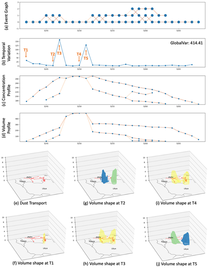
where is the variation calculated between consecutive timestamps t and t+1, as previously defined; t ranges over all timestamps within the event where  and are defined, effectively aggregating the variations from the start to the end of the event. With the data categorized and the temporal dimensions set, the next step is to develop a comprehensive behavioral map or model (Figure 1a). This model visually and conceptually represents how the categorized interactions are interconnected over the defined time frames, illustrating their impact on the system’s overall dynamics. Figure 1a, the Event Graph, serves as a foundational representation, where each point indicates a spatiotemporal event, plotted over time. The y-axis represents the event depth or intensity, while the x-axis indicates the timeline of these occurrences. The lines connecting the points highlight the progression and relationships between these events, offering a clear view of how they unfold over time.

To effectively quantify dynamics, we can calculate the changes in connecting objects’ attributes and spatial locations, including differences in volume, speed and direction, concentration or density, and centroid, as further detailed in Figure 1b through 1d. In addition to these profiles, the spatial characteristics of the events are further explored in Figures 1e through 1j. Figure 1e presents the dust transport, showing the path and spread of dust particles across a geographical area. The 3D representation captures both horizontal and vertical extents, illustrating the movement from a source point and its dispersion across different regions. Figures 1f through 1j depict the volume shapes at key timestamps T1 through T5. These 3D shapes represent the physical volume occupied by the phenomenon at each of these critical moments.

2.3 Implications and Applications

Several examples are described below to showcase how the spatiotemporal data framework can be applied across different fields to enhance understanding, improve predictive accuracy, and inform strategic decisions based on comprehensive analysis of long-term data trends.

The spatiotemporal data framework can be used in tracking environmental changes over extended periods, particularly in identifying and analyzing anomalous climate patterns. For instance, by maintaining a long-term graph database, researchers can detect unusual shifts in temperature trends or precipitation patterns that deviate from historical data. This capability is critical for recognizing early signs of climate change, such as unexpected warming trends or shifts in rainfall distributions, enabling timely policy adjustments and proactive environmental management (Liu et al., 2019; Xue et al., 2023).

In disaster management, the ability to track and analyze the progression of natural disasters such as hurricanes, floods, or wildfires over time is invaluable (Muñoz et al., 2018). The spatiotemporal data framework allows for the creation of detailed models that predict disaster paths and potential impact zones. By understanding the behaviors and triggers of past events, emergency response teams can develop more effective evacuation plans and readiness strategies, significantly reducing potential damage and enhancing community resilience.

References

- Burrough, P.A., McDonnell, R.A., Lloyd, C.D. (2015). Principles of geographical information systems. Oxford University Press, USA.
- Cui, W., Wang, W., Zhang, J., Yang, J. (2019). Multicore structures and the splitting and merging of eddies in global oceans from satellite altimeter data. Ocean Science 15, 413–430.
- Del Mondo, G., RodríGuez, M.A., Claramunt, C., Bravo, L., Thibaud, R. (2013). Modeling consistency of spatio-temporal graphs. Data and Knowledge Engineering, 84, 59–80.
- Foley, J.D. (1996). Computer Graphics: Principles and Practice. Addison-Wesley Professional.
- Galton, A. (2003). Desiderata for a Spatio-temporal Geo-ontology. In: Kuhn, W., Worboys, M.F., Timpf, S. (eds) Spatial Information Theory. Foundations of Geographic Information Science. COSIT 2003. Lecture Notes in Computer Science, vol 2825. Springer, Berlin, Heidelberg.
- Gold, C.M. (2020). Surface interpolation, spatial adjacency and GIS. In: Raper, J. (Ed.), Three Dimensional Applications in GIS. CRC Press.
- Goodchild, M. F. (2004). GIScience, Geography, Form, and Process. Annals of The Association of American Geographers 94, 709–714.
- Hornsby, K. and Egenhofer, M.J. (2000). Identity-based change: a foundation for spatio-temporal knowledge representation. International Journal of Geographical Information Science 14, 207–224.
- Jjumba, A. and Dragićević, S. (2016). A development of spatiotemporal queries to analyze the simulation outcomes from a voxel automata model. Earth Science Informatics 9, 343–353.
- Kaufman, A., and Shimony, E. (1987). 3D scan-conversion algorithms for voxel-based graphics, in: Proceedings of the 1986 Workshop on Interactive 3D Graphics, I3D ’86. Association for Computing Machinery, New York, NY, USA, pp. 45–75.
- Lee, D. T., & Schachter, B. J. (1980). Two algorithms for constructing a Delaunay triangulation. International Journal of Computer & Information Sciences, 9(3), 219-242.
- Liu, J., Xue, C., Dong, Q., Wu, C. and Xu, Y. (2019). A Process-Oriented Spatiotemporal Clustering Method for Complex Trajectories of Dynamic Geographic Phenomena. IEEE Access 7, 155951–155964.
- McIntosh, J. and Yuan, M. (2005). Assessing Similarity of Geographic Processes and Events. Transactions in GIS 9, 223–245.
- Meagher, D. (1982). Geometric modeling using octree encoding. Computer Graphics and Image Processing 19, 129–147.
- Muñoz, C.A., Wang, L.-P., and Willems, P. (2018). Enhanced object-based tracking algorithm for convective rain storms and cells. Atmospheric Research 201, 144–158.
- Peucker, T.K., Fowler, R.J., Little, J.J., and Mark, D.M. (1979). The triangulated irregular network, in: Proc. AutoCarto. pp. 96–103.
- Weibel, R. and Heller, M. (1991). Digital Terrain Modeling. In: Geographical Information Systems: Principles and Applications, London: Longman, pp. 269-297.
- Worboys, M. F. (2005). Event-oriented approaches to geographic phenomena. International Journal of Geographical Information Science, 19 (1), 1–28.
- Xue, C., Niu, C., Xu, Y., & Su, F. (2023). A process-oriented exploration of the evolutionary structures of ocean dynamics with time series of a remote sensing dataset. Remote Sensing, 15, 348.
- Xue, C., Wu, C., Liu, J., and Su, F. (2019). A Novel Process-Oriented Graph Storage for Dynamic Geographic Phenomena. ISPRS International Journal of Geo-Information 8, 100.
- Yi, J., Du, Y., Wang, D., and Zhou, C. (2017). Tracking the evolution processes and behaviors of mesoscale eddies in the South China Sea: a global nearest neighbor filter approach. Acta Oceanologica Sinica 36, 27–37.
- Yu, M. (2020). A Graph-Based Spatiotemporal Data Framework for 4D Natural Phenomena Representation and Quantification–An Example of Dust Events. ISPRS International Journal of Geo-Information 9, 127.
- Yu, M., Yang, C., and Jin, B. (2018). A framework for natural phenomena movement tracking–Using 4D dust simulation as an example. Computers & Geosciences 121, 53–66.
Learning outcomes
-
1732 - Explain the connections between spatiotemporal objects, relations, and events.
Explain the connections between spatiotemporal objects, relations, and events.
1733 - Describe the models that can be used to represent volumes and space-time volumes.
Describe the models that can be used to represent volumes and space-time volumes.
1734 - Illustrate how a spatiotemporal data framework can be used in different application areas.
Illustrate how a spatiotemporal data framework can be used in different application areas.