[DM-01-028] Topological Relationships

Clementini, E. (2025). Topological Relationships. The Geographic Information Science & Technology Body of Knowledge (Issue 2, 2025 Edition), John P. Wilson (Ed.). DOI: 10.22224/gistbok/2025.2.13. 

1. Definitions
2. Overview

1. Definitions

Point-set topology deals with basic set-theoretic definitions related to points of the line, the plane or 3D space. A crucial component of point-set topology is the concept of open set. In fact, a topology is defined as a family of open sets with union and intersection operations. For a formal treatment of topology, we refer to (Munkres, 2014), while in the rest of this chapter we will try to limit the formal definitions to the essentials and accompany them with practical explanations. Informally, an open set is a point-set that do not contain its boundary, and a closed set is a point-set that contains its boundary. An open set is connected if it is possible to draw a line between any two points of the set and all the points in the path belong to the set.

To understand the meaning of the word “topological”, one fundamental notion is the homeomorphism, which is a mathematical transformation that maps near points in one space to near points in another space. Informally, a homeomorphism is a transformation that changes the shape of an object as it were “elastic,” without provoking ruptures or gluing its parts. Therefore, a topological property remains invariant under a homeomorphism. Speaking of relationships between two objects, a topological relationship is unaltered if the scene made up by the two objects undergoes a homeomorphism. In essence, topological relationships capture connection properties of two objects that are invariant even if the objects would change their shape. Formally, the definition of homeomorphism is the following:

Definition 1.1. Let X and Y be two topological spaces. A mapping is a homeomorphism if both  are continuous functions.

Spatial objects, that is, various kinds of points, lines, and regions, need to be precisely defined in geometric terms, in such a way that topological relationships can be calculated without ambiguities. Since various models for topological relationships make use of the fundamental notions of objects’ boundaries and interiors, the latter must be defined as well. In some cases, the adopted GIS definitions deviate from mathematical rigorousness to accommodate practical situations. For example, in topology, a simple line embedded in , being a one-dimensional set, has an empty interior. Following normal practice in both GIS (Egenhofer and Herring, 1990) and in OGC standards (OGC Open Geospatial Consortium Inc., 1999), a line boundary is the set of its end-points and a line interior corresponds to all its points except the end-points. Hence, in this case the GIS definition deviates from mathematics. Let us recap the main definitions, adapted from (Clementini and Di Felice, 1996). Let x be a two-dimensional point-set embedded in .

Definition 1.2. The interior  is the union of all open sets contained in .

Definition 1.3. The closure is the intersection of all closed sets containing .

Definition 1.4. The boundary  is the set difference between its closure and interior, i.e., .

Definition 1.5. The exterior   is the set difference .

Definition 1.6.   is regular closed if 

Definition 1.7. A simple region is a regular closed non-empty two-dimensional point-set  with a connected interior and connected exterior. 

Definition 1.7 implies that a simple region is homeomorphic to the closed unit disk. A simple region does not have holes and is connected. If we omit the constraint of connected exterior from the definition, we obtain regions with holes (Egenhofer et al., 1994):

Definition 1.8.  A region with holes is a regular closed non-empty two-dimensional point-set  with a connected interior.

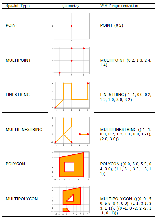
Region with holes are implemented with the Polygon spatial data type in the Open Geospatial Consortium (OGC) simple feature specifications. For the details about the vector data model adopted by the OGC, we refer to the OGC documentation. In this chapter, we limit ourselves to illustrate the OGC spatial data types together with their Well-Known Text (WKT) representation in Table 1.

Table 1. Open Geospatial Consortium (OGC) Spatial Types and their Well-known Text (WKT) Representation. 

Omitting the constraint of a connected interior results in complex regions, i.e., regions with holes and separations: 

Definition 1.9: A complex region is a regular closed non-empty two-dimensional point-set .

The MultiPolygon spatial data type is used in the OGC feature models to implement complex regions.

Definition 1.10. A simple line is a closed non-empty one-dimensional pointset  defined as the image of a continuous mapping  such that .   

Thus a simple line is defined as the mapping of the unit interval in the plane with no self-intersections. Intuitively, a simple line can be constructed by taking a pen and tracing a line on a piece of paper, never passing twice through the same position and never removing the pen until the line is finished.  The initial and final points of a simple line, otherwise called the endpoints of the line, are denoted as . The boundary  of a line  is defined to be the set of its two endpoints, whilst the interior of the line is defined as . Simple lines are implemented with the Linestring spatial data type in the OGC feature model. If the constraint of no self-intersections is removed from Definition 1.10, then we obtain lines with self-intersections, a particular case of which is the closed ring, where:

Definition 1.11. A line with self-intersections is a closed non-empty one-dimensional point-set x defined as the image of a continuous mapping .

A complex line is composed of several components that may be disjoint or not, i.e., the union of several mappings from the unit interval to the plane:

Definition 1.12. A complex line is a closed non-empty one-dimensional pointset x defined as the union of n images of continuous mappings .

Complex lines are implemented with the MultiLinestring spatial data type in the OGC feature model.

Definition 1.13. A simple point is a zero-dimensional element of .

Defintion 1.14. A complex point is a finite set whose elements are simple points.

Following the OGC convention, point features have an empty boundary and they coincide with their interior. The Point and Multipoint spatial data types are used to implement simple and complex point features in OGC standards, respectively.

2. Overview

Various models for representing topological relationships have been published starting from the year 1990. Three of them had major impact: the 9-intersection model (9IM) (Egenhofer and Franzosa 1991) with its dimension extension DE-9IM (Clementini et al. 1993), the Region Connection Calculus (RCC-8) (Cui et al. 1993), and the Calculus Based Method (CBM) (Clementini et al. 1993). We will concentrate on the DE-9IM and the CBM that have been recommended in the OGC specifications. The DE-9IM corresponds to the Relate OGC operator and the CBM corresponds to the OGC named topological relationships (Equals, Disjoint, Intersects, Touches, Crosses, Within, Contains, Overlaps).

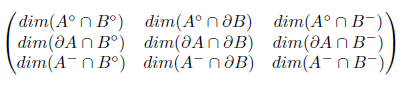
The DE-9IM categorizes topological relationships on the basis of the intersections between interiors, boundaries, and exteriors of two spatial objects A and B, which can be of any type (point, line, or region). The dimension of such intersections are indicated with values −1, 0, 1, 2, corresponding to an empty intersection, a 0-dimensional, 1-dimensional, and 2-dimensional intersection, respectively. The 9 intersections are structured in a 3 × 3 matrix, leading to the following definition:

Definition 2.1.  Given two spatial objects A and B, the DE-91M is the following matrix:

While the matrix can have 4⁹=262144 different values from a combinatorial point of view, only a limited number of values corresponds to actual spatial configurations with 2D geometries. Those configurations can be obtained with a lengthy process by imposing geometric constraints and eliminating the corresponding matrices. The number of possible configurations for simple objects is given in Table 2, distinguishing the type of involved objects.

Table 2. The number of different topological relationships expressible with the DE-9IM for simple spatial objects, distinguished by type: region=R, line=L, point=P.

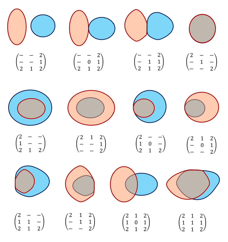
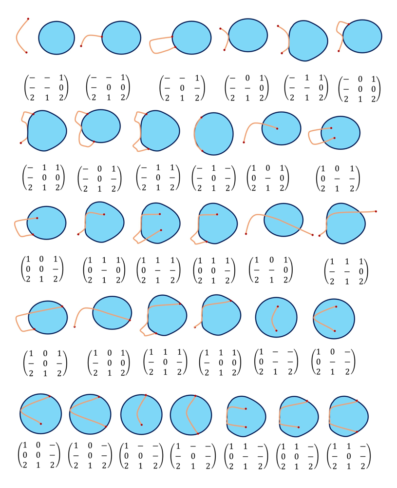
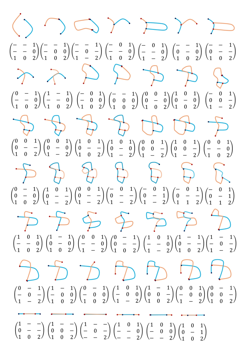
If we consider complex geometries instead, such as regions with holes and separate components, the number of possible relationships is higher. Nobody up to now has calculated the number of possible relationships for complex features that is expressible with the 9I+DEM matrix. In the following figures, we illustrate the relationships for simple features. Figure 1 illustrates the 12 prototypes of topological relationships between simple regions. Figure 2 represents the 31 DE-9IM different relationships between a simple line and a simple region. Figure 3 represents the 48 DE-9IM different relationships between two simple lines.

The CBM provides five names of topological relationships that apply to categories of configurations involving two spatial objects, plus three boundary operators that in combination with the relationship names allow the formulation of logical expressions able to capture a variety of topological aspects. It has been proved equivalent to the DE-9IM in the sense that every DE-9IM matrix can be expressed by a CBM logical expression and, vice versa, every CBM relationship can be expressed by a set of DE-9IM matrices (Clementini and DiFelice, 1995). Given two spatial objects A and B, the CBM definitions are the following:

Definition 2.2. The touch relationship is defined as: 

Definition 2.3. The in relationship is defined as: 

Definition 2.4. The cross relationship is defined as:   

Definition 2.5. The overlap relationship is defined as: 

Definition 2.6. The disjoint relationship is defined as: 

Definition 2.7. Given a region A and a line L, the boundary operators are defined as:  

The OGC named topological relationships (Equals, Disjoint, Intersects, Touches, Crosses, Within, Contains, Overlaps) correspond to the CBM as follows:

Touches (A, B) ⇔ touch (A, B)

Within (A, B) ⇔ in (A, B)

Crosses (A, B) ⇔ cross (A, B)

Overlaps (A, B) ⇔ overlap (A, B)

Disjoint (A, B) ⇔ disjoint (A, B)

Contains (A, B) ⇔ in (B, A)

Equals (A, B) ⇔ in (A, B)  in (B, A)

Intersects (A, B) ⇔ ¬disjoint (A, B)

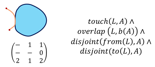
Let us make an example to illustrate how the CBM works. Consider the fifth case on the upper row of Figure 2. To describe such a topological configuration with a CBM expression, we say that the line is touching the region and that at the same time the line is overlapping the region’s boundary and the line’s endpoints are disjoint from the region. Compare the DE-9IM matrix and the CBM logical expression in Figure 4.

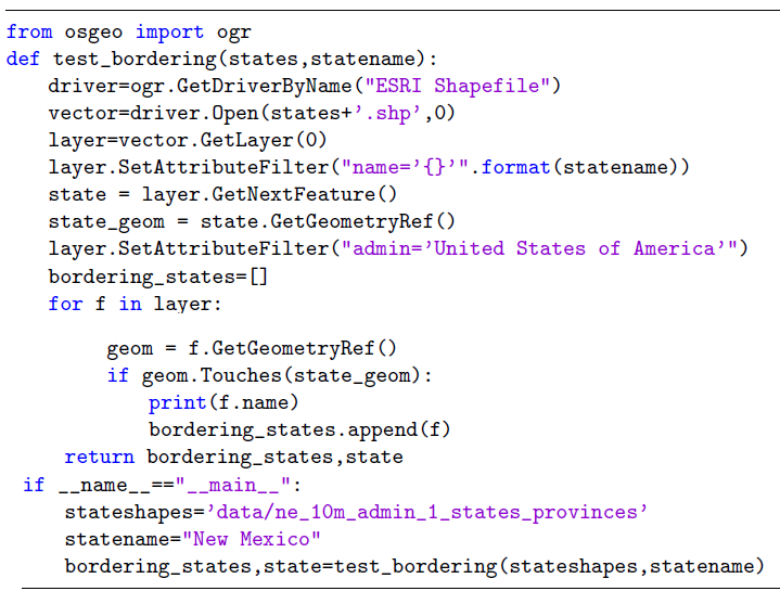
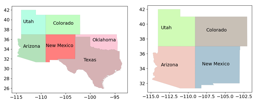
To bridge from the definitions into practice, it is useful to include some instances of sample code in OGC standard. In the following, the first program finds the US states bordering on New Mexico by using the Touches relationship (see graphical output in Figure 5a). The Python code uses the OGR GDAL library for the management of geographic data and the implementation of topological relationships (see https://gdal.org). The dataset is taken from Natural Earth (see https://www.naturalearthdata.com).

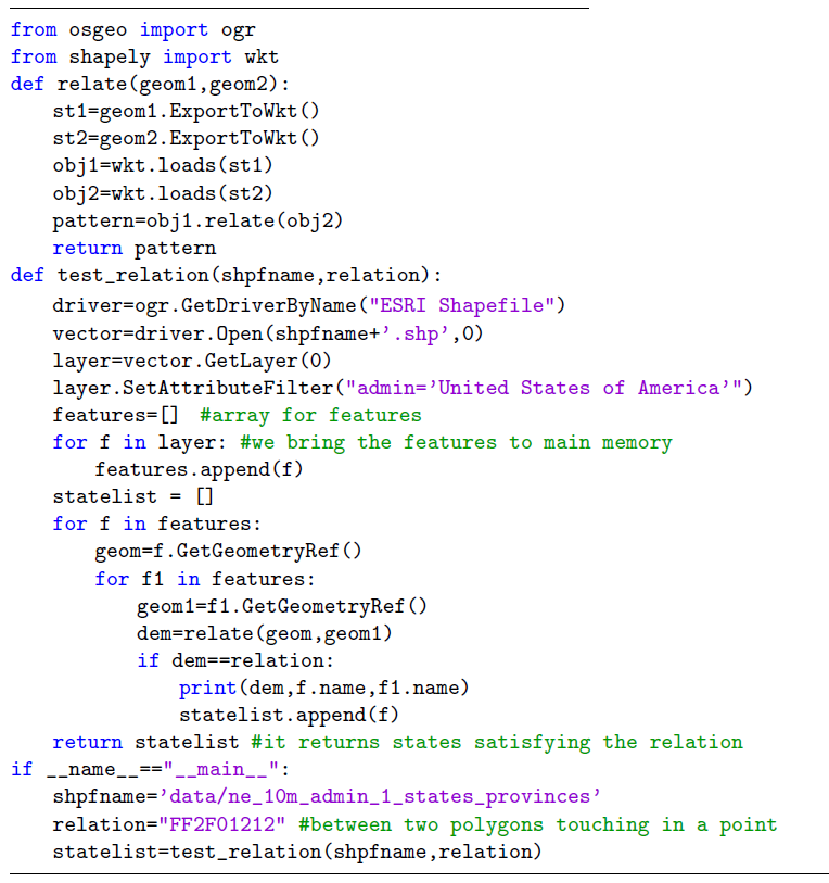
The Relate operator implements the DE-9IM. To illustrate its use, let us find the US states that are bordering on a single point. The DE-9IM relationship that holds when two polygons touch in a point is evaluated by the Relate operator with the string “FF2F01212” (see graphical output in Figure 5b).

Since the OGR GDAL library does not implement the Relate operator, it is necessary to include the ‘shapely’ library as well (see https://shapely.readthedocs.io/en/ 2.0.6/manual.html), as follows.

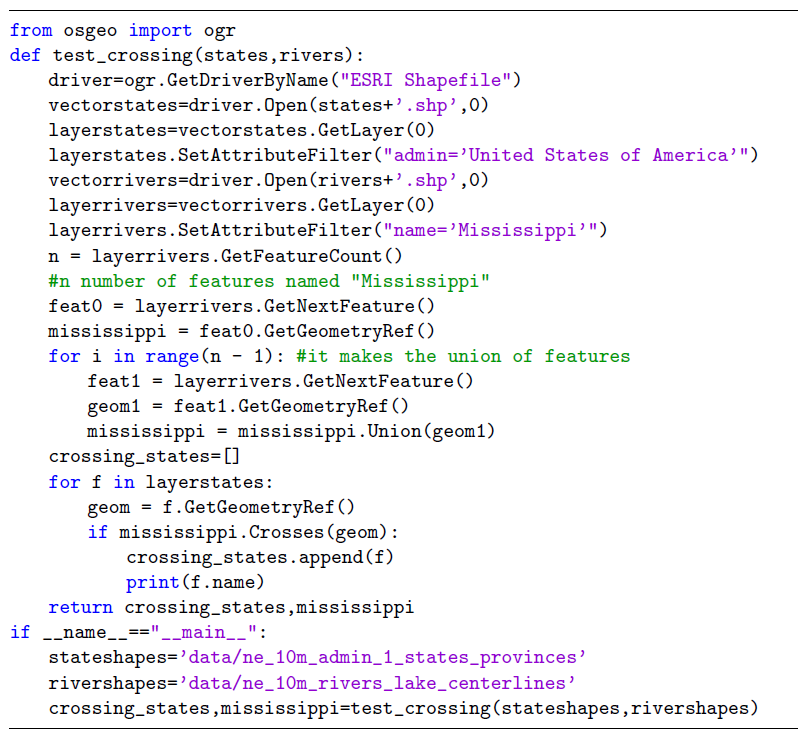
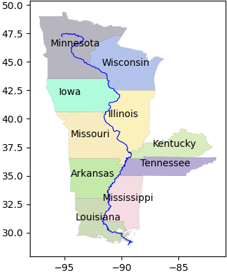
A third sample code is about topological relationships between polygons and polylines. We show the use of the Crosses relationship to find out the US states crossed by the river Mississippi. In the Natural Earth dataset, as it is quite common with linear shapes, the river Mississippi is represented by more than a single feature. Therefore, as a first step it is necessary to make the geometric union of all the features with name Mississippi to obtain a single MultiPolyline representing the river. After that, with the the Crosses relationship, we can check the states that are crossed by the river. See the following program and the graphical output in Figure 6.

The study of topological relationships is a fascinating research topic that has produced many different results, broken down into different application fields. Despite efforts, the potential of the topic has not been fully exploited yet, especially regarding the extensions to 3D space and to objects with uncertain boundaries.

References

- Clementini, E. and Di Felice, P. (1995). A comparison of methods for representing topological relationships. Information Sciences - Applications, 3(3):149–178.
- Clementini, E. and Di Felice, P. (1996). A Model for Representing Topological Relationships Between Complex Geometric Features in Spatial Databases. Information Sciences, 90 (1-4):: 121-136.
- Clementini, E., Di Felice, P., van Oosterom, P. (1993). A small set of formal topological relationships suitable for end-user interaction. In: Abel, D., Chin Ooi, B. (eds) Advances in Spatial Databases. SSD 1993. Lecture Notes in Computer Science, vol 692. Springer, Berlin, Heidelberg
- Cui, Z., Cohn, A. G., and Randell. D. A. (1993). Qualitative and Topological Relationships in Spatial Databases. In Proceedings of the Third International Symposium on Advances in Spatial Databases (SSD '93). Springer-Verlag, Berlin, Heidelberg, 296–315.
- Egenhofer, M. J. and Herring, J. R. (1990). Categorizing binary topological relations between regions, lines and points in geographic databases. In The 9- Intersection: Formalism and Its Use for Natural-Language Spatial Predicates. National Center for Geographic Information and Analysis, University of California, Santa Barbara, CA.
- Egenhofer, M. J., & Franzosa, R. D. (1991). Point-set Topological Spatial Relations. International Journal of Geographical Information System, 5(2), 161-174.
- Egenhofer, M. J., Clementini, E., & di Felice, P. (1994). Topological relations between regions with holes. International Journal of Geographical Information Systems, 8(2), 129–142.
- Munkres, J. (2014). Topology, 1st Edition. Pearson Education Limited.
- Open Geospatial Consortium (OGC). (2011). OpenGIS Implementation Standard for Geographic information - Simple feature access - Part 1: Common architecture. OGC 06-103r4, Open Geospatial Consortium Inc.
Learning outcomes
-
1943 - Define the most widespread models for describing topological relationships.
1944 - Identify the correct topological relationship in a geometric scene of two spatial objects.
1945 - Describe a topological relationship in either the DE-9IM or the CBM models.