[FC-06-011] Set Theory

Arlinghaus, S. L. (2019). Set Theory. The Geographic Information Science & Technology Body of Knowledge (2nd Quarter 2019 Edition), John P. Wilson (Ed.). DOI: 10.22224/gistbok/2019.2.1

This Topic is also available in the following editions:  

DiBiase, D., DeMers, M., Johnson, A., Kemp, K., Luck, A. T., Plewe, B., and Wentz, E. (2006). Set theory. The Geographic Information Science & Technology Body of Knowledge. Washington, DC: Association of American Geographers. (2nd Quarter 2016, first digital)

1. Classical Set Theory: a Brief View and Definitions
2. GIS and Set Theory: Three Examples
3. Beyond Basic Set Theory: Directions

1. Classical Set Theory: a Brief View and Definitions

Much of mathematics, including set theory, rests on the Law of the Excluded Middle: For any given Proposition, either the Proposition is True, or its negation is True. Statements are "true" or "false."  Unlike the real world, much of the mathematical world is based on a two-valued logic system. There is no "compromise" —things are right or wrong, clearly. This difference between the real and the mathematical world makes for a continuing, and interesting, challenge in linking the two.   

The focus in this chapter is on foundations as they arise directly from pure mathematics:  in particular from set theory, which is itself foundational within all of a twentieth century (and later) view of mathematics. The notion of "set" has been around as long as human beings have. Euclid and early mathematicians employed ideas about sets. But, set theory, as a defined discipline, did not emerge until Georg Cantor characterized it more formally in the latter part of the nineteenth century (Cantor, 1874, 1915).  Early appreciation of it came only from within pure mathematics.   

Set theory's rich, compact history mirrors the somewhat linear nature of the development of a standard of mathematics curriculum in which there are clear patterns in time and sequencing of what material precedes, or follows, other material. Set theory is at the heart of, or a first step to, many of those sequences. It is also at the heart of GIS.

• The concept of a set. The concept of a set is natural; it is what the reader thinks it is: a well-defined collection or grouping of elements. “Well-defined” simply means that there is no ambiguity as to whether any given element belongs to the grouping or does not belong to the grouping. An intuitive appreciation of it is relatively easily acquired (Halmos, 1960). Generally, all members of a given set share a common characteristic; thus, it becomes  straightforward to identify elements that are, or are not, members of a given set. For example, there is a set of even positive integers and a set of odd positive integers. These two sets have no members in common. 
• Binary relation.  Set theory begins with intuitive assumptions. It posits a binary relation between an object o and a set A. If o is an element of A, the notation o ∈ A is used to denote membership of o in A. Indeed, as arithmetic is based on binary operations on numbers, set theory is based on binary operations on sets.
• Set notation.  When displaying sets by enumerating members, it is conventional to enclose the members in braces:  {1, 2, 3} or {2, 4, 6, …} with ellipsis used to denote continuation in pattern. A more abstract, but compact, notation is to express a set as {a | a ∈ X} or {a : a ∈ X}  to be read as "the set of all a such that a is an element of X."
• Relations among sets:  subsets.  Sets, themselves, may also be viewed as objects; thus, the membership relation can relate sets to each other. A binary relation between two sets is the subset relation, or set inclusion. If all the members of set A are also members of set B, then A is a subset of B, denoted A ⊆ B. For example, {0,1} is a subset of {-1, 0, 1} , while {1, 2} is not. Or, the set of even positive integers is a subset of the set of positive integers. The full, given, set is a subset of itself (hence the equal sign on the inclusion symbol).  If the full set is to be excluded from the set of subsets, then we use the term, proper subset, for cases where only subsets smaller than the full set are considered (and notationally, the equals part of the symbol is removed).   
• Two special sets.  There are two special sets that come up often. The importance of zero in arithmetic, also has a parallel in set theory with the empty (or null) set (a set of 0 elements), denoted ∅. The empty set is one special set. The other is the "universe of discourse" or the "universal set" or the universe." The universal set might be denoted as U, or some other symbol where context makes the designation obvious. Here, too, there are parallels with basic arithmetic where the "universe" might be considered as the set of all positive integers or some other infinite set. The universal set serves as a context within which analysis takes place.
• Basic Binary Set Operations
  • 1.1. Union.  The union of the sets A and B, denoted A ∪ B, is the set of all objects that are members of A, or of B, or of both.  For example, {1, 2, 3} ∪ {2, 4, 6} = {1, 2, 3, 4, 6}. 
  • 1.2. Intersection.  The intersection of the sets A and B, denoted A ∩ B, is the set of all objects that are members of both A and B.  For example, {1, 2, 3} ∩ {2, 4, 6} = {2}.  If the intersection of two sets has no elements in common, the intersection is the empty set, and the two sets are said to be disjoint.
  • 1.3. Set difference; set complements
    • Absolute difference:  Given the universal set U and a subset A within U. The difference of U and A, denoted U - A, is the set of all members of U that are not members of A. This set is also called the complement of A in U, denoted Ac. For example, suppose U = {all positive integers} and A = {all positive integers divisible by 3} = {3, 6, 9, 12, …}. Then, U - A = (all positive integers that are not divisible by 3} = {1, 2, 4, 5, 7, 8, 10, 11, 13, …}.
    • Relative difference:  Given sets A and B within a universal set U. The difference of B and A, denoted B - A, is the set of all members of B that are not members of A.  It might also be referred to as the complement of A relative to B.  For example, suppose U is the set of all rational numbers (integers and non-integer fractions), A is the set of all positive integers, and B is the set of all positive rational numbers.  Then B – A is the set of positive non-integer fractions.
  • 1.4. Symmetric difference.  The symmetric difference of sets A and B, denoted A △ B, is the set of all objects that are a member of exactly one of A or B, but not both. For example, the symmetric difference of the set of rational numbers and the set of positive integers is the set of positive non-integer fractions together with zero and the negative rational numbers.
  • 1.5. Cartesian product (Figure 1).  The Cartesian product (named for French Philosopher and Mathematician, René Descartes) of A and B, denoted A × B, is the set whose members are all possible ordered pairs (a, b) where a is a member of A and b is a member of B.  The familiar coordinatized plane of analytic geometry is simply the Cartesian product of the real numbers, R, with itself:  R x R.  There are various views one might have of representing a Cartesian product. As a real world example, a deck of standard playing cards becomes the Cartesian product of the set of thirteen alphanumeric symbols 2,3,4,5,6,7,8,9, A, K, Q, J, with the set of four suit symbols ♣, ♦, ♥, ♠ for a total of 13 x 4 = 52 ordered pairs represented on 52 cards (e.g., 10 of diamonds; queen of spades; or ace of hearts).

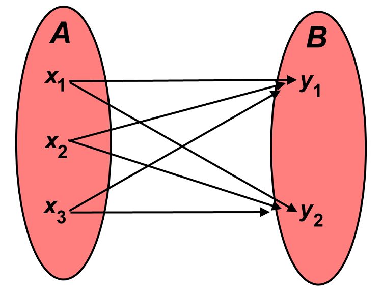
Figure 1. Cartesian product of two sets A and B:  A = {x1, x2, x3}, B={y1, y2} and A × B = {(x1, y1), (x1, y2), (x2, y1), (x2, y2), (x3, y1), (x3, y2)}.  Source: author. 

• • 1.6. Power set.  The power set of a set A is the set whose members are all possible subsets of A, including the empty set and the entire set itself.  For example, the power set of {1, 2} is { { }, {1}, {2}, {1, 2} } . The “Hasse” diagram below, Figure 2, shows a systematic method for hierarchically enumerating all members of the power set of {1, 2, 3, 4}. 

Figure 2. Hasse diagram showing an hierarchical pattern for enumerating all subsets of the set A = {1,2,3,4}, the power set of A.  Source: author. 

2. GIS and Set Theory: Three Examples

2.1 Story Maps

Maps tell stories. Set theory might be viewed as an abstract underpinning to such stories. One set of maps that folks often follow is the set of seasonal influenza maps of the Centers for Disease Control in the USA (see CDC reference). They tell the story of the spread, by state, of influenza, on a week by week basis, across the USA. States are shaded by level of influenza activity from "No Activity" to "Sporadic" to "Local Activity" to "Regional" to "Widespread." The states, as spatial entities have no overlap. They are disjoint sets, when viewed as areas.  But, if one counts boundary lines, do adjacent states share a common boundary?  What is the definition of "state" and what are its criteria for existence? There may be philosophical issues in understanding and communication; or, as Smith and Mark have put it, "Do Mountains Exist?" (2003). What do the colors for these categories represent?  Each indicates that a threshold number of members of the set has the flu.  What is that threshold number?  Might it be characterized in set notation?  Where does the idea of "subset" fit in?  Are there pockets within a given state in which the level of flu activity is different in a small area from what it is in the entire state?  A college campus with many students living in dormitories might experience flu activity different from the state-wide activity level.  What other unseen set-theoretic  concepts might lurk in maps? The abstract concepts presented in the first section can find application and interpretation in countless ways in the world of mapping as well as in the world of mathematics.

2.2 Venn Diagrams and Municipal Planning

Municipal planners may take preference surveys of various sorts to assist them in optimizing resource allocation, access to services, or other municipal issues. Such surveys may be part of the foundation of mapped results shown to Planning Commissioners and City Council representatives who ultimately decide what gets funded and moves forward. Having clear displays of complicated data sets can be critical to success.

Suppose the results of a survey, involving commuting preference to the downtown showed, that during the past three days, there were 7000 individuals who were asked to say if they had used any or all of train, bus, or car for their commute. The results, stated partially, were as follows:

• Train:  4700 people had used the train, and of those, 1400 had also used a car for at least one trip (but not the bus), while 800 of those 4700 had used both a car and a bus for at least one trip.
• Bus:  3100 people had used the bus, and of those, 500 had also used the train for at least one trip (but not a car), while 800 of those 3100 had used both a car and a train for at least one trip.
• Car:  2900 people had used a car, and of those, 200 had also used the bus for at least one trip (but not the train), while 800 of those 2900 had used both a bus and a train for at least one trip.

While it appears that there might be useful information from this survey, it is difficult to detect pattern in displays of data such as the one above.  To aid with visualization and to help understand patterns in the data in advance of mapping, a 3-circle Venn diagram is useful. 

Let one circle represent "car," another represent "train," and another represent "bus."  Draw them in a pretzel configuration inside a rectangle to maximize overlap in eight distinct areas, including outside the pretzel but inside the rectangle. The rectangle represents the universe of discourse, in this case "three-day commuting modes used."

To fill in the data, put the value of 800 in the region that lies in the center of the pretzel, contained in each of the three large circles: the intersection of the circles representing all three transit modes. Next, fill in each of the remaining pieces for intersections of pairs of sets. Finally, calculate the values for the remaining single-mode regions from information already present. The result is the Venn diagram in Figure 3.

Figure 3. Venn diagram showing survey results for commuter preference among available modes over a three-day period.  The symbol U indicates the Universe containing the set pattern.  The color selection represents ideas of color mixing.  For example, white, in the intersection of all circles, is the presence of all colors while black, outside the RGB circles, and CMY intersections, represents the absence of color.  Note other subtleties, such as color selection in the outlining of text, as well. Source: author. 

It is easier to grasp pattern from the diagram than from the enumeration of data. Beyond that, the Venn diagram is compact and the display can easily be shared with other municipal authorities and members of the public. Furthermore, percentages are easy to calculate: for example, one can read off that 4,700 out of 7,000 took the train over a three day period which is about 67 percent. Planners, and those questioning planners, might wish to have information such as that at their fingertips (on their smart phones) when plans for parking garages, train stations and stops, as well as access to rights of way, come up for discussion and eventual evaluation. Venn diagrams can organize and efficiently display large amounts of information in a quick and accurate manner with consequent use for additional analysis.

2.3 The Word "Or"

The English word "or" is an interesting one. It's such a simple word but has been the source of much unintended confusion over many years. The problem lies in its two different forms: "inclusive" and "exclusive" forms. Inclusive "or" means either A or B or both (as in 1.1, set union) whereas exclusive "or" means either A or B but not both (as in 1.4, symmetric difference). 

Scholars accustomed to reading legal texts and various other formal, logical texts may think that "or" is generally exclusive. However, in set theory and anything based on it, the word 'or' is typically used in its inclusive form: one or the other or both. In the setting of GIS software, elementary students often have problems with this distinction, perhaps when performing joins or for various other reasons. The instructor wishing to save his/her own time, and prevent student frustration, is probably well-advised, early in the course, to explain the difference between "inclusive or" and "exclusive or" and to note, verbally, when it arises in later sections of material.

3. Beyond Basic Set Theory: Directions

3.1 Cardinality and One-to-one Correspondence

Cardinality is a measure of the number of elements in a set. In finite sets, simple counting can determine the cardinality.  The cardinality of the deck of playing cards, generated above as a Cartesian product, is 52.  To compare the size of two sets, A and B, employ the following strategy:

• If the two sets are finite, simply count the number of elements in each, if reasonable, and compare the answers to see if they are the same size.
• Find a relationship between sets A and B such that each element of A corresponds to exactly one element of B and each element of B corresponds to exactly one element of A. This relationship is called a one-to-one correspondence (Birkhoff and Mac Lane, 1941).  If there exists a one-to-one correspondence between A and B, then they have the same cardinality, denoted |A| = |B|. This general, systematic process holds for all sets, finite and infinite, but it is the only process that applies to infinite sets.

3.2 Counting (ℵ0)

3.2.1 Positive integers and positive even integers. 

Consider the following question:  which set is larger...the set of positive integers (natural numbers) or the set of even positive integers (those divisible by the number 2)?  Use the concept of one-to-one correspondence to find the cardinality of each set, A = {1, 2, 3, 4, …n,…} and B = {2, 4, 6, 8,…2n,…}.  Mapping n to 2n exhibits the pattern; each element of A maps to exactly one element of B (twice its size) and each element of B maps to exactly one element of A (half its size). Because the sets are infinite, the numbers never "run out." Here, an infinite set has the same cardinality as a proper subset of itself!  Cantor called the "transfinite" number, representing the cardinality of the set of natural numbers (the smallest order of infinity), aleph null, denoted ℵ0.  Because the ‘natural’ numbers are commonly used as "counting" numbers, an infinite set that can be put into one-to-one correspondence with the natural numbers is called a "countable" set. Such sets all have cardinality aleph null.

3.2.2 Natural Numbers and Rational Numbers

A similar question involves asking if there is a one-to-one correspondence between the set of natural numbers, N and the rational numbers (fractions) Q (think "quotient").  From an intuitive standpoint, it appears that the set of rational numbers must be larger than the natural numbers. There are an infinite number of rational numbers between two consecutive natural numbers and there are no natural numbers between the same two consecutive natural numbers. Again, Cantor found a one-to-one correspondence between N and a set containing Q to show that |N| = |Q| = ℵ0. Cantor’s argument that the set of rational numbers is countable can be visualized, in more than one way, using a diagonalization technique (Stones, 2014).

3.3 On beyond ℵ0

In both examples of the previous section, an infinite set and a proper infinite subset of it, were put into one-to-one correspondence.  One might wonder if all that was needed was to be sufficiently clever in ordering elements to show that any infinite set is countable. And, if such were the case, then how could there be transfinite numbers beyond ℵ0.  Indeed, part of the research associated with set theory in the late nineteenth and twentieth centuries, continuing to today, dealt with the issue of sets with cardinality beyond ℵ0.

3.3.1 Dedekind Cuts and Real Numbers

Richard Dedekind, a contemporary of Cantor, worked in the late nineteenth century on strategies for formal characterization of the such ideas and found Cantor's set theory to be critical in enunciating them.  A Dedekind Cut (Schnitt) of the rational numbers is a partition of the set Q into two nonempty subsets S1 and S2 such that all members of S1 are less than those of S2 and such that S1 has no greatest member (Dedekind, 1901 in 1963). Consider the set S2:

• If S2 has a smallest element that is a rational number, then that cut corresponds to that rational number.
• If S2 does not have a smallest element that is a rational number, then that cut defines a unique irrational number. One might think of it as filling a gap between S1 and S2.  

An irrational cut is assigned an irrational number which is in neither S1 nor S2.  A real number is equated to exactly one cut of rationals, thus composing the set of real numbers as the set of rational numbers together with the set of irrational numbers. Cantor used an argument, similar to the one he used with countability of the rational numbers, to show that the set of real numbers is larger than the set of rationals: it is "uncountable."  For more detail and references, see for example Cantor’s Diagonal Method (Weisstein, 1999-2018).  Thus, the number line, on which every real number is defined as a Dedekind cut of the set of rational numbers, is a continuum with no gaps.

3.3.2 The Continuum

The Continuum Hypothesis, first proposed by Georg Cantor, suggests that the cardinal number of the continuum is the same as that of aleph1 which is greater than aleph null (ℵ0) and questions whether there is another transfinite number between these two (Cohen, 1966). The remarkable truth, which has occupied decades of scholars, is that this proposition is undecidable, since neither it nor its converse contradicts the basic tenets of set theory (and may depend on the version of set theory employed).  Indeed, since it was first proposed by Cantor, the validity of the Continuum Hypothesis, has occupied over 100 years of research in the Foundations of Mathematics.

3.3.3 GIS and the Continuum

Any coordinate system of the Earth's surface, associated with its mapping, makes use of the fact that there are no gaps in the real number line:  a direct application of Cantor's and Dedekind's work on the cardinality of the real numbers. Lack of gaps is a fact, however, that mapping experts generally take for granted and may not think about at all. If there were gaps in the axes by which geographic spaces were coordinatized, then there would be holes in the map where there should be land or water. Without the "no gaps" real number line, mapping would be radically different. Of course, for centuries people used the real number line perhaps without thinking about its properties. Cantor and Dedekind changed that--it is important to acknowledge that in fact it is certain that there are no gaps--not just assume that there are no gaps because it looks as if there are no gaps. Cantor also demonstrated quite aptly that trusting intuition, when dealing with the infinite, is a risky business.

3.3.4 Peano Space-filling Curves

The focus, above, in comparing sizes of infinite sets, is on exhibiting one-to-one correspondences in a numerical context. It is natural also to ask equivalent questions geometrically.  Thus, are there more points in a plane than there are on a line?  As with thinking about the size of the set of rational numbers in relation to the set of natural numbers, it would seem natural to think that of course there are more points in the plane than on the line. 

Giuseppe Peano, another contemporary of Cantor's, introduced space-filling curves that he used to define a one-to-one correspondence from a line to a plane area. His systematic process develops a curve that twists in a predictable and replicable manner to fill space (Peano, 1890). The process involves scaling of an initial curve that is repeated, in a predictable infinite manner, to fill an area. His construction suggests that the set of points on the side of a square lies in one-to-one correspondence with the set of points in the area of the square.  From there, it is not a long leap to see that the number of points on the real number line is the same as the number of points in the two-dimensional plane.

3.3.5 Space-filling and Fractals

Peano’s space-filling curves very quickly become difficult to draw and to imagine.  In fact, they remained fairly well hidden throughout much of the 20th century, to almost all but those interested in the Foundations of Mathematics.  After the development of high-speed computing, Benoit Mandelbrot and others employed the vast power of mid-twentieth century (and later) technology to create clear, and beautiful, pictures of the Peano-type curves and related geometric entities (Mandelbrot, 1982).  Mandelbrot coined the term "fractals" (short for "fractional dimension") for these, and related, curves that were formed from infinite self-replication with scale adjustment, reminiscent of the style of Peano. This latter process, he called "self-similarity." Unlike the situation for the continuum, where people had been using the material for centuries without grasping transfinite numbers and cardinal arithmetic, here contemporary technology appeared necessary to bring to life a grand idea from the past. The fractal represents a true interactive win-win achievement between theory and practice.

By the end of the 20th century, applications of fractals in the physical, the biological, and the social sciences had become abundant. They were prevalent in popular culture as pictures on calendars, on postcards, in artwork, and so forth.  Fractals appeared in the geographical literature that centered on physical geographical applications as well as on urban and other geographical applications (Mandelbrot, 1982; Arlinghaus, 1985; Arlinghaus and Arlinghaus, 1989; Batty and Longley, 1994).  The concept of fractals, derived from set theory, has served as a rich and rewarding research area for many in the GIS world.

3.3.6 The Cantor Set

One fractal form, from Cantor's work, is his set of excluded middle thirds, often referred to simply as the Cantor Set. This set unifies much of the history of set theory and its role leading from the time of Cantor to the present. It captures the Law of the Excluded Middle, the real number line as the Continuum, uncountability and countability, the space-filling curves of Peano, self-similarity and fractals, as well as some other deep properties. 

The Cantor Set is created by deleting, iteratively, the open middle third from a set of line segments (that is, open middle thirds are line segments with no endpoints). Figure 4 illustrates the process through the first six steps, geometrically (Barlie and Weisstein, 1999-2018). Notationally, begin with the closed interval [0, 1].  Delete the open middle third (1/3, 2/3). The two line segments [0, 1/3] ∪ [2/3, 1] remain. Next delete the middle third of each of these, leaving four line segments. Continue the process infinitely, creating smaller and smaller segments with an eventual "dust"-like appearance. The final set contains all points in the interval [0, 1] that are not deleted in the infinite process. The Cantor set exhibits self-similarity, because it is equal to two copies of itself, if each copy is shrunk by a factor of 3 and translated.

Figure 4. Cantor Set.  Excluded middle thirds of segments, displayed through six steps. Source:  Wikimedia Commons.

The Cantor set is defined as the set of points that remain after the infinite exclusion process. Thus, the amount of the unit interval that remains can be found by subtracting the total length removed. That removed total is given by the geometric series 1/3 + 2/9 + 4/27 + 8/81 +... = 1/3(1/(1-2/3)) = 1. Thus, what is left is 1-1 = 0. So, this set cannot contain any interval of non-zero length. 

However, the geometric process illustrates that there are an infinite number of points remaining, the endpoints of the removed intervals. The construction steps to create the Cantor set are countable in number so the number of endpoints remaining, from the excluded thirds, are also countable in number. In addition, there are also other points that remain that are not endpoints but that never get excluded because they are never inside a middle third. The number 1/4 is such an example (think back to Dedekind cuts). Thus, the Cantor set has no line segments remaining, but it has a countable number of points generated as endpoints in the process as well as an uncountable number of other points that never appear in deleted thirds (most of the elements of the Cantor set). The entire Cantor set, as a "dust," is uncountable.

One doesn't often see direct application of Cantor's Set in the GIS world—at least not yet.  Where one sees it more, as seems to be the case with much of set theory and other elements of pure mathematics, is in its foundational role within pure mathematics. Glimpses from other parts of set theory offer exciting hints and challenges toward future research directions.  With such "foundational" thoughts, we have now come full-circle from the beginning of this chapter: from one excluded middle to another!

1. Fuzzy sets:  between true and false. 
   1. Weisstein, E. W.  (1999-2018).  Fuzzy logic.  MathWorld—A Wolfram Web Resource, retrieved from http://mathworld.wolfram.com/FuzzyLogic.html
   2. Hwang, S and Thill, J-C. (2004).  Modeling Localities with Fuzzy Sets and GIS, In: Cobb M, Petry F, and Robinson V (eds) Fuzzy Modeling with Spatial Information for Geographic Problems, Springer-Verlag:  71-104.
2. Graph theory:  Abstract network forms.
   1. Harary, F. (1969). Graph Theory.  Boston:  Addison-Wesley.
   2. Arlinghaus, S. L.; Arlinghaus, W. C., and Harary, F.  (2002).  Graph Theory in Geography:  An Interactive View, eBook.  New York, NY:  Wiley-Interscience Series in Discrete Mathematics and Optimization, John Wiley and Sons.
3. Point-set topology:  generalized pure mathematics linking set theory and connectivity, compactness, and related topics. 
   1. Kelley, J. L. (1955). General Topology.  Princeton, NJ:  D. Van Nostrand Company Inc.
   2. Chiang, M. and Yang, M. (2004). Towards Network X-ities from a Topological Point of View:  Evolvability and Scalability.  Proc. 42nd Allerton Conference.
4. Category theory:  A possible alternative foundational world.
   1. Mac Lane, S. (1998). Categories for the Working Mathematician. Graduate Texts in Mathematics. 5 (2nd ed.). Springer-Verlag. 
   2. Arlinghaus, S. and Kerski, J. (2015).  Category Theory in Geography?  Quaestiones Geographicae, 34(4), 61-68. 
5. Selected publication lists:
   1. Albrecht, J.  Publication list, retrieved from http://www.geo.hunter.cuny.edu/~jochen/
   2. Tobler, W.  Publication list, retrieved from https://www.geog.ucsb.edu/~tobler/publications/index.html

References

- Abbott, E. A. (1884). Flatland: A Romance of Many Dimensions. London: Seeley & Co.
- Arlinghaus, S. L. (1985). Fractals Take a Central Place. Geografiska Annaler, Series B, Human Geography, 67(2), 83-88.
- Arlinghaus, S. L. and Arlinghaus, W. C. (1989). The fractal theory of central place geometry: a Diophantine analysis of fractal generators for arbitrary Löschian numbers. Geographical Analysis: An International Journal of Theoretical Geography, 21(2), 103-121.
- Barile, M. and Weisstein, E. W. (1999-2023). Cantor Set. MathWorld—A Wolfram Web Resource.
- Batty, M. and Longley, P. (1994). Fractal Cities: A Geometry of Form and Function. San Diego, CA and London, UK: Academic Press.
- Birkhoff, G. and MacLane, S. (1941). A Survey of Modern Algebra. New York, NY: MacMillan.
-
Cantor, G. (1955) [1915]. P. Jourdain, ed. Contributions to the Founding of the Theory of Transfinite Numbers. New York, NY: Dover Publications.
Cantor, G. (1955) [1915]. P. Jourdain, ed. Contributions to the Founding of the Theory of Transfinite Numbers. New York, NY: Dover Publications. - Cantor, H. (1984). Ueber eine Eigenschaft des Inbegriffes aller reellen algebraischen Zahlen. In: Über unendliche, lineare Punktmannigfaltigkeiten. Teubner-Archiv zur Mathematik, vol 2. Springer, Vienna
- Carroll, L. (1895). What the Tortoise Said to Achilles. Mind 4, No. 14 (April 1895): 278-280.
- Centers for Disease Control (CDC). (2018). Weekly US Map: Influenza Summary Update.
- Cohen, P. (2008). Set Theory and the Continuum Hypothesis. Reprint of the 1966 Edition. New York, NY: Dover Publications.
- Dedekind, R. (1963). Continuity and Irrational Numbers. Essays on the Theory of Numbers. New York, NY: Dover Publications.
- Esri. (n.d.). How to Make a Story Map. Last retrieved 2018.
- Halmos, P. (1960). Naïve Set Theory. Princeton, NJ: D. Van Nostrand Company.
- Herstein, I. N. (1964). Topics in Algebra. New York: Blaisdell.
- Mandelbrot, B. B. (1983). The Fractal Geometry of Nature. New York: W.H. Freeman.
- Mansfield, M. (1963). Introduction to Topology. Princeton, NJ: D. Van Nostrand Company.
- Peano, G. (1890). Sur une courbe, qui remplit toute une aire plane, Mathematische Annalen (in French), 36 (1): 157–160.
- Smith, B. and Mark, D. M. (2003). Do Mountains Exist? Towards an Ontology of Landforms. Environment and Planning B: Urban Analytics and City Science, 30(3).
- Stones, R. J. (2014). How to prove that Q (the rationals) is a countable set. MathStack Exchange.
- Weisstein, E. W. (n.d.). Cantor Diagonal Method. From MathWorld--A Wolfram Web Resource.
Learning outcomes
64 - Compare and contrast basic set theory and basic arithmetic.
Compare and contrast basic set theory and basic arithmetic.
86 - Compare and contrast logic and set theory
Compare and contrast logic and set theory
157 - Conjecture where else you might wish to see set theory used in GIS.
Conjecture where else you might wish to see set theory used in GIS.
476 - Describe set theory
Describe set theory
678 - Describe where you already know that set theory is used in existing GIS software
Describe where you already know that set theory is used in existing GIS software
Related topics
Additional resources